March 16, 2021

tabulizer Rocks

Voter Turnout in Oregon

Oregon’s voter turnout data is published by the Oregon Secretary of State’s office. You can find a direct link to the .pdf here. How hard is to recover a .pdf table? Let’s see. I am going to work with tabulizer.

library(tabulizer)
library(dplyr)

The key function for this will be extract_tables; with knowledge of that let’s see if it just automagically works.

library(kableExtra)
location <- 'https://sos.oregon.gov/elections/Documents/Voter_Turnout_History_General_Election.pdf'
out <- extract_tables(location)
head(out) %>% kable() %>% scroll_box(height="300px")

Year	Total Registered Voters	Total Votes Cast	% of Turnout
2020	2,951,428	2,317,965	78.50%
2018	2,763,105	1,873,891	67.80%
2016	2,553,808	2,051,452	80.33%
2014	2,174,763	1,541,782	70.90%
2012	2,199,360	1,820,507	82.80%
2010	2,068,798	1,487,210	71.89%
2008	2,153,914	1,845,251	85.67%
2006	1,976,669	1,399,650	70.81%
2004	2,141,249	1,851,671	86.48%
2002	1,872,615	1,293,756	69.09%
2000	1,954,006	1,559,215	79.80%
1998	1,965,981	1,160,400	59.02%
1996	1,962,155	1,399,180	71.31%
1994	1,832,774	1,254,265	68.44%
1992	1,775,416	1,462,314	82.36%
1990	1,476,500	1,133,125	76.74%
1988	1,528,478	1,235,199	80.81%
1986	1,502,244	1,088,140	72.43%
1984	1,608,693	1,265,824	78.69%
1982	1,516,589	1,063,913	70.15%
1980	1,569,222	1,209,691	77.09%
1978	1,482,339	937,423	63.20%
1976	1,420,146	1,048,561	73.83%
1974	1,143,073	792,557	69.34%
1972	1,197,676	953,376	79.60%
1970	955,459	671,878	70.32%
1968	971,851	824,562	84.84%
1966	949,825	693,796	73.04%
1964	932,461	791,245	84.86%
1962	883,690	644,772	72.96%
1960	900,627	779,159	86.51%

So far so good. Now a bit of wrangling in two steps. First, I need to get rid of the first row. Second, I need to get rid of the percent signs and commas.

library(stringr)
Cleaned <- out %>% data.frame() %>% 
  filter(X1!="Year") %>% 
  transmute(year = as.numeric(X1), 
            RegVoters = as.numeric(str_remove_all(X2, ",")), 
            Votes = as.numeric(str_remove_all(X3, ",")), 
            Vote.Percent = as.numeric(str_remove(X4, "%")))
Cleaned %>% head() %>% kable() %>% scroll_box(height="300px")

year	RegVoters	Votes	Vote.Percent
2020	2951428	2317965	78.50
2018	2763105	1873891	67.80
2016	2553808	2051452	80.33
2014	2174763	1541782	70.90
2012	2199360	1820507	82.80
2010	2068798	1487210	71.89

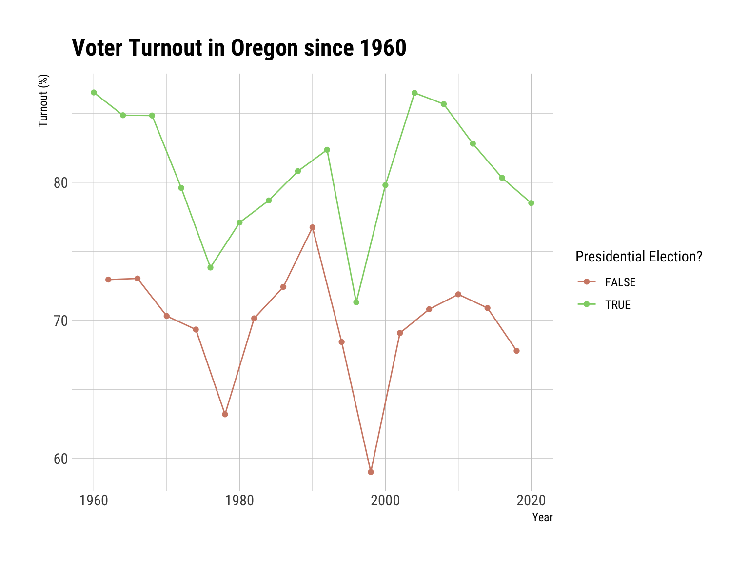
One more relevant feature is that midterms and presidential years are a bit different so let me denote this with an indicator. The method I will use is does the integer division of year minus 1960 divided by four have no remainder [TRUE] or have a remainder [FALSE].

library(fpp3); library(magrittr); library(hrbrthemes)
Cleaned %<>% mutate(President = as.factor(((year - 1960) %% 4) == 0))

Now I have exactly the dataset that I want. What does the plot look like?

Cleaned %>% ggplot(.) + aes(x=year, y=Vote.Percent, color=President, group=President) + geom_point() + geom_line() + scale_color_ipsum() + labs(title="Voter Turnout in Oregon since 1960", x="Year", y="Turnout (%)", color="Presidential Election?") + theme_ipsum_rc()