slider is a magical way of creating moving averages
Nike’s Stock
# Load libraries
library(tidyquant)
library(tidyverse)
library(fpp3)
With those libraries, I should have what I need. Let me get Nike’s stock from 2015.
# Get Nike stock data
Nike.Stocks <- tq_get("NKE", from="2015-01-01")
Nike.Stocks %>% as_tsibble(index=date) %>% autoplot(adjusted) + labs(y="Adjusted Closing Price", title="NKE since 2015")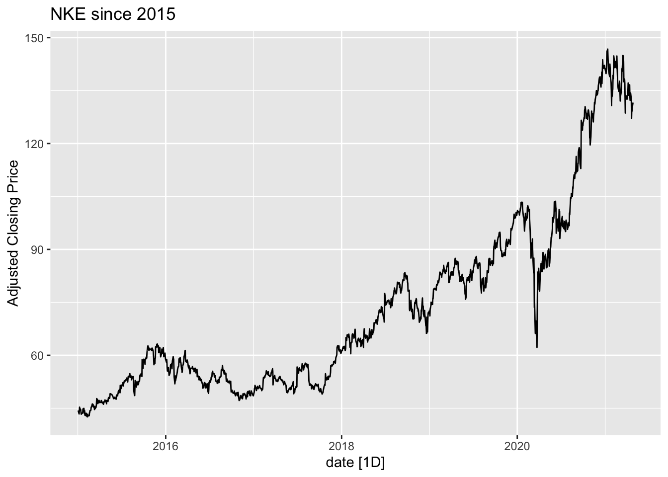
Now I want to create monthly data. I will the yearmonth type from lubridate. By default, tidyquant uses yearmon which is different.
# Create nike returns, need tq_transmute because we are taking daily data and turning it into monthly.
Nike.Returns <- Nike.Stocks %>% tq_transmute(adjusted, mutate_fun=periodReturn, period="monthly")
Nike.Returns # It is monthly but the date is a date.  To make them match, I need a yearmonth
## # A tibble: 76 x 2
## date monthly.returns
## <date> <dbl>
## 1 2015-01-30 -0.0293
## 2 2015-02-27 0.0558
## 3 2015-03-31 0.0331
## 4 2015-04-30 -0.0149
## 5 2015-05-29 0.0314
## 6 2015-06-30 0.0625
## 7 2015-07-31 0.0667
## 8 2015-08-31 -0.0301
## 9 2015-09-30 0.103
## 10 2015-10-30 0.0655
## # … with 66 more rowsI want to mutate the date to be a yearmonth. Getting the time measure right is the crucial part of this.
Nike.Returns <- Nike.Returns %>% mutate(date = yearmonth(date))
Nike.Returns
## # A tibble: 76 x 2
## date monthly.returns
## <mth> <dbl>
## 1 2015 Jan -0.0293
## 2 2015 Feb 0.0558
## 3 2015 Mar 0.0331
## 4 2015 Apr -0.0149
## 5 2015 May 0.0314
## 6 2015 Jun 0.0625
## 7 2015 Jul 0.0667
## 8 2015 Aug -0.0301
## 9 2015 Sep 0.103
## 10 2015 Oct 0.0655
## # … with 66 more rowsNow let me try another mutation. Let me keep the last closing price of the month. The last step here makes sure the dates are the same type. All of this remains tibble as the type; not tsibble. That is convenient for joining data.
Nike.Last <- Nike.Stocks %>%
  tq_transmute(select = adjusted, mutate_fun = to.monthly)
Nike.Last
## # A tibble: 76 x 2
## date adjusted
## <yearmon> <dbl>
## 1 Jan 2015 43.0
## 2 Feb 2015 45.5
## 3 Mar 2015 47.0
## 4 Apr 2015 46.3
## 5 May 2015 47.7
## 6 Jun 2015 50.7
## 7 Jul 2015 54.1
## 8 Aug 2015 52.4
## 9 Sep 2015 57.9
## 10 Oct 2015 61.6
## # … with 66 more rowsThat is not quite right. This is a yearmon type. I need to change that.
Nike.Last <- Nike.Last%>%
  mutate(date = yearmonth(date))
Nike.Last
## # A tibble: 76 x 2
## date adjusted
## <mth> <dbl>
## 1 2015 Jan 43.0
## 2 2015 Feb 45.5
## 3 2015 Mar 47.0
## 4 2015 Apr 46.3
## 5 2015 May 47.7
## 6 2015 Jun 50.7
## 7 2015 Jul 54.1
## 8 2015 Aug 52.4
## 9 2015 Sep 57.9
## 10 2015 Oct 61.6
## # … with 66 more rowsThe dates match up in type now, so they should join up nicely. Let’s try that.
Nike.Data <- Nike.Returns %>% left_join(., Nike.Last, by = c("date" = "date"))
Nike.Data
## # A tibble: 76 x 3
## date monthly.returns adjusted
## <mth> <dbl> <dbl>
## 1 2015 Jan -0.0293 43.0
## 2 2015 Feb 0.0558 45.5
## 3 2015 Mar 0.0331 47.0
## 4 2015 Apr -0.0149 46.3
## 5 2015 May 0.0314 47.7
## 6 2015 Jun 0.0625 50.7
## 7 2015 Jul 0.0667 54.1
## 8 2015 Aug -0.0301 52.4
## 9 2015 Sep 0.103 57.9
## 10 2015 Oct 0.0655 61.6
## # … with 66 more rowsThe next step is to turn it into a tsibble. That means defining the yearmonth as the data and indexing a tsibble by that.
Nike.Data <- Nike.Data %>% mutate(date = yearmonth(date)) %>% as_tsibble(index=date)Now it is a tsibble to work with in the fpp3 workflow. Finally, let’s set up training and test sets. Working with the Nike data; use filter_index to grab all the data up to and including January 2020
Nike.Data.Train <- Nike.Data  %>% filter_index(. ~ "2020-01")
# Look at it.
Nike.Data.Train %>% tail()
## # A tsibble: 6 x 3 [1M]
## date monthly.returns adjusted
## <mth> <dbl> <dbl>
## 1 2019 Aug -0.0152 83.3
## 2 2019 Sep 0.111 92.6
## 3 2019 Oct -0.0465 88.3
## 4 2019 Nov 0.0467 92.4
## 5 2019 Dec 0.0836 100.
## 6 2020 Jan -0.0495 95.2# Create a test set as everything that is not in the training set, e.g. the last 15 months
Nike.Data.Test <- anti_join(Nike.Data,Nike.Data.Train) %>% as_tsibble(index=date)
Nike.Data.Test## # A tsibble: 15 x 3 [1M]
## date monthly.returns adjusted
## <mth> <dbl> <dbl>
## 1 2020 Feb -0.0693 88.6
## 2 2020 Mar -0.0743 82.0
## 3 2020 Apr 0.0537 86.4
## 4 2020 May 0.134 98.0
## 5 2020 Jun -0.00538 97.4
## 6 2020 Jul -0.00449 97.0
## 7 2020 Aug 0.149 111.
## 8 2020 Sep 0.122 125.
## 9 2020 Oct -0.0435 120.
## 10 2020 Nov 0.122 134.
## 11 2020 Dec 0.0524 141.
## 12 2021 Jan -0.0557 133.
## 13 2021 Feb 0.0110 135.
## 14 2021 Mar -0.0140 133.
## 15 2021 Apr -0.00971 132.The Forecasting Workflow
Nike.Mods <- Nike.Data.Train %>%
  model(
    ARIMA(monthly.returns),
    ETS(monthly.returns))
Nike.Mods %>% forecast(h=12) %>% accuracy(Nike.Data.Test)
## # A tibble: 2 x 10
## .model .type ME RMSE MAE MPE MAPE MASE RMSSE ACF1
## <chr> <chr> <dbl> <dbl> <dbl> <dbl> <dbl> <dbl> <dbl> <dbl>
## 1 ARIMA(monthly.retur… Test 0.0174 0.0828 0.0737 148. 148. NaN NaN 0.0130
## 2 ETS(monthly.returns) Test 0.0174 0.0828 0.0737 148. 148. NaN NaN 0.0130A plot.
Nike.Mods %>% forecast(h=12) %>% autoplot() + geom_point(data=Nike.Data.Test, aes(x=date, y=monthly.returns)) + facet_wrap(vars(.model)) + guides(level=FALSE, color=FALSE, fill=FALSE) + theme_minimal()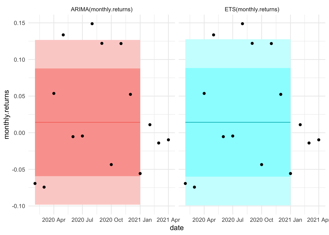
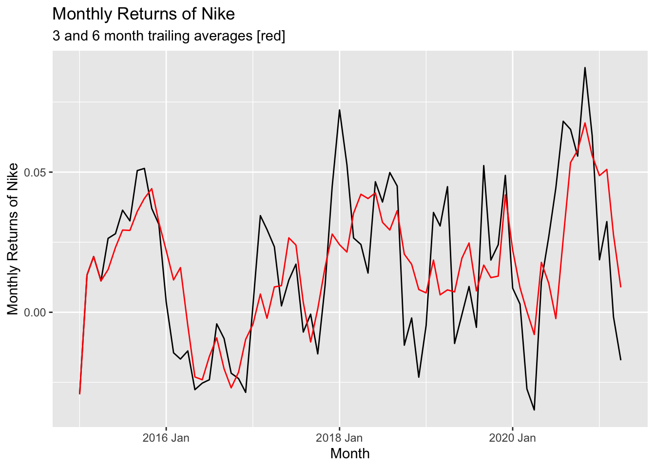
Three-month trailing averages
NMA <- Nike.Data %>% mutate(MMR3 = slider::slide_dbl(monthly.returns, mean, .before=3, .after=0), MMR6 = slider::slide_dbl(monthly.returns, mean, .before=6, .after=0))
NMA %>% autoplot(MMR3) + autolayer(NMA %>% select(MMR6), color="red") + labs(x="Month", y="Monthly Returns of Nike", title="Monthly Returns of Nike", subtitle="3 and 6 month trailing averages [red]")