ARCH and GARCH Models
NKE
First, let me use tidyquant to acquire the data.
library(tidyquant); library(tidyverse)
NKE <- tq_get("NKE", from="2019-01-01")
NKE
## # A tibble: 918 × 8
## symbol date open high low close volume adjusted
## <chr> <date> <dbl> <dbl> <dbl> <dbl> <dbl> <dbl>
## 1 NKE 2019-01-02 72.8 74.6 72.2 74.1 6762700 71.7
## 2 NKE 2019-01-03 73.2 73.3 71.2 72.8 8007400 70.4
## 3 NKE 2019-01-04 73.4 75.1 73.1 74.7 7844200 72.3
## 4 NKE 2019-01-07 74.7 76.4 74.3 75.7 8184800 73.3
## 5 NKE 2019-01-08 76.8 77.4 76.2 76.7 8809000 74.3
## 6 NKE 2019-01-09 77.0 77.2 76.1 76.6 8591000 74.2
## 7 NKE 2019-01-10 75.6 77.3 75.5 76.4 11148600 74.0
## 8 NKE 2019-01-11 76.3 76.9 75.8 76.0 10689900 73.6
## 9 NKE 2019-01-14 75.5 76.8 75.5 76.1 5677400 73.7
## 10 NKE 2019-01-15 76.2 78.0 76.1 77.9 6212400 75.4
## # … with 908 more rowsFor a variety of reasons, equities are unlikely to be mean-reverting in level form. Let me apply some unit-root testing for Nike since 2019.
NKEAC <- NKE %>% select(date, adjusted)
summary(urca::ur.df(NKEAC$adjusted))
##
## ###############################################
## # Augmented Dickey-Fuller Test Unit Root Test #
## ###############################################
##
## Test regression none
##
##
## Call:
## lm(formula = z.diff ~ z.lag.1 - 1 + z.diff.lag)
##
## Residuals:
## Min 1Q Median 3Q Max
## -9.938 -1.044 0.067 1.168 20.568
##
## Coefficients:
## Estimate Std. Error t value Pr(>|t|)
## z.lag.1 0.0001009 0.0006328 0.160 0.873
## z.diff.lag -0.0012145 0.0330807 -0.037 0.971
##
## Residual standard error: 2.269 on 914 degrees of freedom
## Multiple R-squared: 2.903e-05, Adjusted R-squared: -0.002159
## F-statistic: 0.01326 on 2 and 914 DF, p-value: 0.9868
##
##
## Value of test-statistic is: 0.1595
##
## Critical values for test statistics:
## 1pct 5pct 10pct
## tau1 -2.58 -1.95 -1.62summary(urca::ur.df(NKEAC$adjusted, type="trend"))##
## ###############################################
## # Augmented Dickey-Fuller Test Unit Root Test #
## ###############################################
##
## Test regression trend
##
##
## Call:
## lm(formula = z.diff ~ z.lag.1 + 1 + tt + z.diff.lag)
##
## Residuals:
## Min 1Q Median 3Q Max
## -9.8038 -1.0576 -0.0166 1.0902 20.6120
##
## Coefficients:
## Estimate Std. Error t value Pr(>|t|)
## (Intercept) 5.575e-01 3.425e-01 1.628 0.104
## z.lag.1 -4.600e-03 4.014e-03 -1.146 0.252
## tt 3.295e-05 4.383e-04 0.075 0.940
## z.diff.lag 1.013e-04 3.320e-02 0.003 0.998
##
## Residual standard error: 2.267 on 912 degrees of freedom
## Multiple R-squared: 0.003104, Adjusted R-squared: -0.0001755
## F-statistic: 0.9465 on 3 and 912 DF, p-value: 0.4175
##
##
## Value of test-statistic is: -1.1461 1.0607 1.4188
##
## Critical values for test statistics:
## 1pct 5pct 10pct
## tau3 -3.96 -3.41 -3.12
## phi2 6.09 4.68 4.03
## phi3 8.27 6.25 5.34summary(urca::ur.df(NKEAC$adjusted, type = "drift"))##
## ###############################################
## # Augmented Dickey-Fuller Test Unit Root Test #
## ###############################################
##
## Test regression drift
##
##
## Call:
## lm(formula = z.diff ~ z.lag.1 + 1 + z.diff.lag)
##
## Residuals:
## Min 1Q Median 3Q Max
## -9.8025 -1.0509 -0.0196 1.0868 20.6135
##
## Coefficients:
## Estimate Std. Error t value Pr(>|t|)
## (Intercept) 0.5462463 0.3075563 1.776 0.0761 .
## z.lag.1 -0.0043702 0.0025955 -1.684 0.0926 .
## z.diff.lag -0.0001219 0.0330476 -0.004 0.9971
## ---
## Signif. codes: 0 '***' 0.001 '**' 0.01 '*' 0.05 '.' 0.1 ' ' 1
##
## Residual standard error: 2.266 on 913 degrees of freedom
## Multiple R-squared: 0.003098, Adjusted R-squared: 0.0009138
## F-statistic: 1.418 on 2 and 913 DF, p-value: 0.2426
##
##
## Value of test-statistic is: -1.6837 1.59
##
## Critical values for test statistics:
## 1pct 5pct 10pct
## tau2 -3.43 -2.86 -2.57
## phi1 6.43 4.59 3.78summary(urca::ur.kpss(NKEAC$adjusted, type = "mu"))##
## #######################
## # KPSS Unit Root Test #
## #######################
##
## Test is of type: mu with 6 lags.
##
## Value of test-statistic is: 9.2369
##
## Critical value for a significance level of:
## 10pct 5pct 2.5pct 1pct
## critical values 0.347 0.463 0.574 0.739summary(urca::ur.kpss(NKEAC$adjusted, type = "tau"))##
## #######################
## # KPSS Unit Root Test #
## #######################
##
## Test is of type: tau with 6 lags.
##
## Value of test-statistic is: 1.411
##
## Critical value for a significance level of:
## 10pct 5pct 2.5pct 1pct
## critical values 0.119 0.146 0.176 0.216So the process seems to clearly contain a unit-root, statistically. Let’s have a look.
Visualizing Adjusted Close
library(fpp3)
NKE %>% mutate(tday = row_number()) %>% as_tsibble(index=tday) %>% autoplot(adjusted)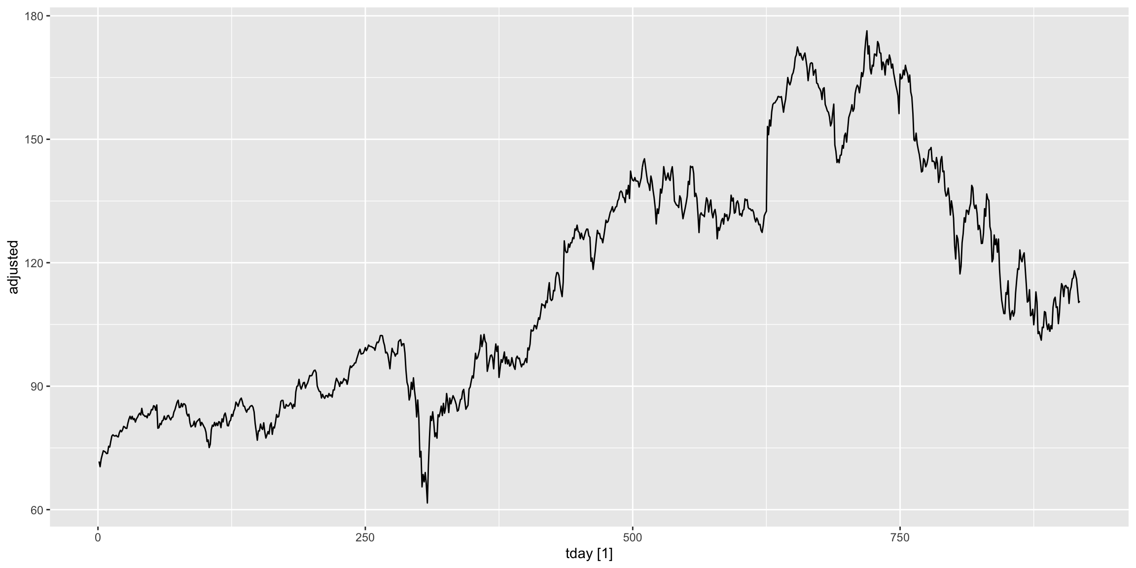
Returns
Let me work with returns.
NKER <- NKE %>% tq_transmute(select=adjusted, mutate_fun = periodReturn, period="daily") %>% mutate(tday = row_number())
NKER %>% as_tsibble(index=tday) %>% autoplot(daily.returns)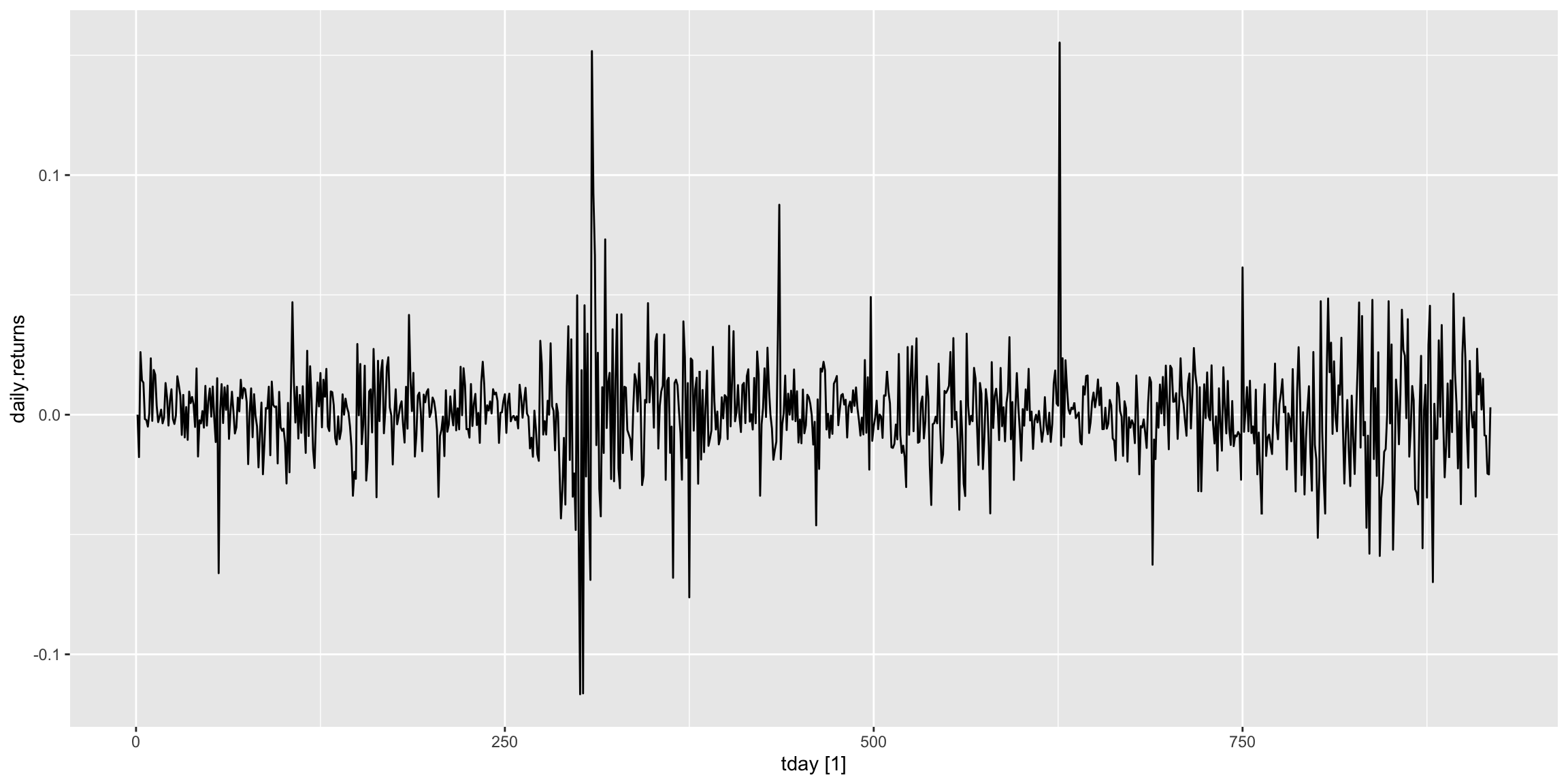
Unit roots and returns
How do the returns seem to behave?
summary(urca::ur.df(NKER$daily.returns))##
## ###############################################
## # Augmented Dickey-Fuller Test Unit Root Test #
## ###############################################
##
## Test regression none
##
##
## Call:
## lm(formula = z.diff ~ z.lag.1 - 1 + z.diff.lag)
##
## Residuals:
## Min 1Q Median 3Q Max
## -0.118677 -0.008654 0.000554 0.011048 0.155177
##
## Coefficients:
## Estimate Std. Error t value Pr(>|t|)
## z.lag.1 -0.97198 0.04690 -20.726 <2e-16 ***
## z.diff.lag -0.03425 0.03307 -1.036 0.301
## ---
## Signif. codes: 0 '***' 0.001 '**' 0.01 '*' 0.05 '.' 0.1 ' ' 1
##
## Residual standard error: 0.02064 on 914 degrees of freedom
## Multiple R-squared: 0.504, Adjusted R-squared: 0.5029
## F-statistic: 464.4 on 2 and 914 DF, p-value: < 2.2e-16
##
##
## Value of test-statistic is: -20.7258
##
## Critical values for test statistics:
## 1pct 5pct 10pct
## tau1 -2.58 -1.95 -1.62summary(urca::ur.df(NKER$daily.returns, type="trend"))##
## ###############################################
## # Augmented Dickey-Fuller Test Unit Root Test #
## ###############################################
##
## Test regression trend
##
##
## Call:
## lm(formula = z.diff ~ z.lag.1 + 1 + tt + z.diff.lag)
##
## Residuals:
## Min 1Q Median 3Q Max
## -0.119867 -0.009244 -0.000428 0.009998 0.155032
##
## Coefficients:
## Estimate Std. Error t value Pr(>|t|)
## (Intercept) 2.135e-03 1.370e-03 1.558 0.120
## z.lag.1 -9.774e-01 4.701e-02 -20.791 <2e-16 ***
## tt -3.148e-06 2.582e-06 -1.219 0.223
## z.diff.lag -3.158e-02 3.311e-02 -0.954 0.340
## ---
## Signif. codes: 0 '***' 0.001 '**' 0.01 '*' 0.05 '.' 0.1 ' ' 1
##
## Residual standard error: 0.02063 on 912 degrees of freedom
## Multiple R-squared: 0.5054, Adjusted R-squared: 0.5037
## F-statistic: 310.6 on 3 and 912 DF, p-value: < 2.2e-16
##
##
## Value of test-statistic is: -20.7914 144.0971 216.1456
##
## Critical values for test statistics:
## 1pct 5pct 10pct
## tau3 -3.96 -3.41 -3.12
## phi2 6.09 4.68 4.03
## phi3 8.27 6.25 5.34summary(urca::ur.df(NKER$daily.returns, type = "drift"))##
## ###############################################
## # Augmented Dickey-Fuller Test Unit Root Test #
## ###############################################
##
## Test regression drift
##
##
## Call:
## lm(formula = z.diff ~ z.lag.1 + 1 + z.diff.lag)
##
## Residuals:
## Min 1Q Median 3Q Max
## -0.119360 -0.009343 -0.000130 0.010387 0.154500
##
## Coefficients:
## Estimate Std. Error t value Pr(>|t|)
## (Intercept) 0.0006866 0.0006828 1.006 0.315
## z.lag.1 -0.9742361 0.0469504 -20.750 <2e-16 ***
## z.diff.lag -0.0331021 0.0330908 -1.000 0.317
## ---
## Signif. codes: 0 '***' 0.001 '**' 0.01 '*' 0.05 '.' 0.1 ' ' 1
##
## Residual standard error: 0.02064 on 913 degrees of freedom
## Multiple R-squared: 0.5045, Adjusted R-squared: 0.5035
## F-statistic: 464.9 on 2 and 913 DF, p-value: < 2.2e-16
##
##
## Value of test-statistic is: -20.7503 215.2877
##
## Critical values for test statistics:
## 1pct 5pct 10pct
## tau2 -3.43 -2.86 -2.57
## phi1 6.43 4.59 3.78summary(urca::ur.kpss(NKER$daily.returns, type = "mu"))##
## #######################
## # KPSS Unit Root Test #
## #######################
##
## Test is of type: mu with 6 lags.
##
## Value of test-statistic is: 0.2047
##
## Critical value for a significance level of:
## 10pct 5pct 2.5pct 1pct
## critical values 0.347 0.463 0.574 0.739summary(urca::ur.kpss(NKER$daily.returns, type = "tau"))##
## #######################
## # KPSS Unit Root Test #
## #######################
##
## Test is of type: tau with 6 lags.
##
## Value of test-statistic is: 0.0648
##
## Critical value for a significance level of:
## 10pct 5pct 2.5pct 1pct
## critical values 0.119 0.146 0.176 0.216So we can reject the null of a unit root and we fail to reject the null of stationarity of the returns. How about the correlation functions?
ACF and PACF of Returns
NKER %>% as_tsibble(index=tday) %>% gg_tsdisplay(daily.returns, plot_type = "partial")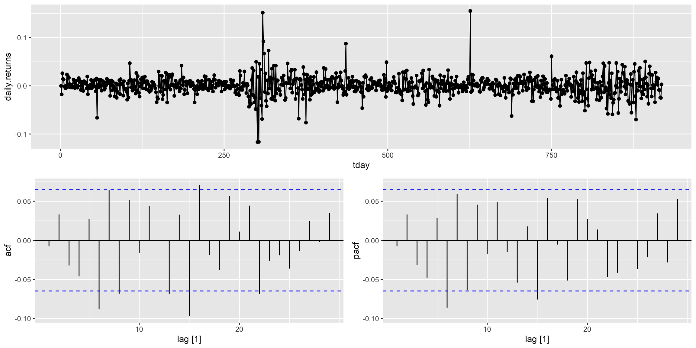
They are nominally white noise.
Box.test(NKER$daily.returns, type = "Ljung-Box")##
## Box-Ljung test
##
## data: NKER$daily.returns
## X-squared = 0.052508, df = 1, p-value = 0.8188NKER %>% as_tsibble(index=tday) %>% model(ARIMA(daily.returns)) %>% report()## Series: daily.returns
## Model: ARIMA(0,0,0)
##
## sigma^2 estimated as 0.000425: log likelihood=2260.79
## AIC=-4519.57 AICc=-4519.57 BIC=-4514.75So the returns have a slightly positive and marginally significant constant. Nike has averaged 0.15 percent returns per day over the period given this very simple representation.
Models
Let’s start with a representation of an AR(p) process.
\[R_{t} = \mu_{R} + \phi_{1}R_{t-1} + \phi_{2}R_{t-2} + \ldots + \phi_{p}R_{t-p} + \epsilon_{t} \]
where
\[ \mathbb{E}[\epsilon_{t}] = 0 \]
and
\[ \mathbb{E}[\epsilon \epsilon^{\prime}] = \sigma^{2} \cdot I_{T} \]
where \(R_{t}\) represent the returns at time \(t\), \(\mu\) is the mean of the stationary process generating \(R_{t}\) and \(\epsilon\) is a white noise error term. Note the stationarity of \(R_t\) is arises so long as the roots of \(1 - \phi_{1}z + \phi_{2}z^2 + \ldots + \phi_{p}z^{p} = 0\) and that the unconditional variance is constant.
ARCH(m)
The ARCH(m) process of Engel (1982) describes the square of \(\epsilon_{t}\) to follow an AR(m) process such that \[ \epsilon_{t}^{2} = \xi + a_{1}\epsilon_{t-1}^{2} + a_{2}\epsilon_{t-2}^{2} + \ldots + a_{m}\epsilon_{t-m}^{2} + \omega_{t} \] with \(\omega\) as white noise. The \(\epsilon\) are errors in forecasting \(R\); the same restriction on the roots will apply from before. The unconditional variance is still a constant described now by \(\frac{\xi}{1-a_{1}-a_{2}-\ldots-a_{m}}\).
There are a few implementations of the basic test for ARCH effects. Let’s have a look at one through six lags. I am not going to tidy this.
1:6 %>% map(function(x) {FinTS::ArchTest(NKER$daily.returns, lags = x)})## [[1]]
##
## ARCH LM-test; Null hypothesis: no ARCH effects
##
## data: NKER$daily.returns
## Chi-squared = 37.705, df = 1, p-value = 8.23e-10
##
##
## [[2]]
##
## ARCH LM-test; Null hypothesis: no ARCH effects
##
## data: NKER$daily.returns
## Chi-squared = 66.435, df = 2, p-value = 3.747e-15
##
##
## [[3]]
##
## ARCH LM-test; Null hypothesis: no ARCH effects
##
## data: NKER$daily.returns
## Chi-squared = 66.504, df = 3, p-value = 2.392e-14
##
##
## [[4]]
##
## ARCH LM-test; Null hypothesis: no ARCH effects
##
## data: NKER$daily.returns
## Chi-squared = 66.651, df = 4, p-value = 1.155e-13
##
##
## [[5]]
##
## ARCH LM-test; Null hypothesis: no ARCH effects
##
## data: NKER$daily.returns
## Chi-squared = 72.462, df = 5, p-value = 3.147e-14
##
##
## [[6]]
##
## ARCH LM-test; Null hypothesis: no ARCH effects
##
## data: NKER$daily.returns
## Chi-squared = 97.817, df = 6, p-value < 2.2e-16The evidence suggests the presence of ARCH effects. Let’s model them. For this, we need a way to represent these models in a consistent syntax.
ARCH
options(scipen=7)
NKER.arch <- tseries::garch(NKER$daily.returns,c(0,1))
##
## ***** ESTIMATION WITH ANALYTICAL GRADIENT *****
##
##
## I INITIAL X(I) D(I)
##
## 1 4.037780e-04 1.000e+00
## 2 5.000000e-02 1.000e+00
##
## IT NF F RELDF PRELDF RELDX STPPAR D*STEP NPRELDF
## 0 1 -3.126e+03
## 1 7 -3.127e+03 4.74e-04 7.64e-04 2.8e-04 3.0e+09 2.8e-05 1.16e+06
## 2 8 -3.128e+03 1.92e-05 2.28e-05 2.7e-04 2.0e+00 2.8e-05 1.60e+01
## 3 15 -3.144e+03 5.14e-03 8.32e-03 4.5e-01 2.0e+00 8.3e-02 1.59e+01
## 4 16 -3.149e+03 1.84e-03 1.44e-03 1.8e-01 0.0e+00 5.6e-02 1.44e-03
## 5 18 -3.154e+03 1.46e-03 1.16e-03 1.9e-01 0.0e+00 8.7e-02 1.16e-03
## 6 19 -3.155e+03 4.06e-04 2.89e-04 9.0e-02 0.0e+00 5.5e-02 2.89e-04
## 7 20 -3.156e+03 1.28e-04 1.04e-04 5.8e-02 0.0e+00 4.1e-02 1.04e-04
## 8 21 -3.156e+03 1.11e-05 9.76e-06 2.1e-02 0.0e+00 1.6e-02 9.76e-06
## 9 22 -3.156e+03 2.95e-07 2.83e-07 3.5e-03 0.0e+00 2.7e-03 2.83e-07
## 10 23 -3.156e+03 7.57e-10 7.66e-10 2.0e-04 0.0e+00 1.5e-04 7.66e-10
## 11 24 -3.156e+03 9.69e-13 1.02e-12 1.1e-06 0.0e+00 8.7e-07 1.02e-12
##
## ***** RELATIVE FUNCTION CONVERGENCE *****
##
## FUNCTION -3.155817e+03 RELDX 1.111e-06
## FUNC. EVALS 24 GRAD. EVALS 12
## PRELDF 1.018e-12 NPRELDF 1.018e-12
##
## I FINAL X(I) D(I) G(I)
##
## 1 2.798850e-04 1.000e+00 2.490e-01
## 2 3.900802e-01 1.000e+00 4.005e-05summary(NKER.arch)##
## Call:
## tseries::garch(x = NKER$daily.returns, order = c(0, 1))
##
## Model:
## GARCH(0,1)
##
## Residuals:
## Min 1Q Median 3Q Max
## -5.71023 -0.45067 0.04028 0.59324 9.19373
##
## Coefficient(s):
## Estimate Std. Error t value Pr(>|t|)
## a0 0.000279885 0.000006364 43.981 <2e-16 ***
## a1 0.390080215 0.039840355 9.791 <2e-16 ***
## ---
## Signif. codes: 0 '***' 0.001 '**' 0.01 '*' 0.05 '.' 0.1 ' ' 1
##
## Diagnostic Tests:
## Jarque Bera Test
##
## data: Residuals
## X-squared = 3656.1, df = 2, p-value < 2.2e-16
##
##
## Box-Ljung test
##
## data: Squared.Residuals
## X-squared = 0.6779, df = 1, p-value = 0.4103So the model seems to capture the ARCH part in the \(a_{1}\) part as the squared residuals are white noise but the Jarque-Bera test suggests deviations from normality. What about a GARCH process?
NKER.garch <- tseries::garch(NKER$daily.returns,c(1,1))##
## ***** ESTIMATION WITH ANALYTICAL GRADIENT *****
##
##
## I INITIAL X(I) D(I)
##
## 1 3.825265e-04 1.000e+00
## 2 5.000000e-02 1.000e+00
## 3 5.000000e-02 1.000e+00
##
## IT NF F RELDF PRELDF RELDX STPPAR D*STEP NPRELDF
## 0 1 -3.128e+03
## 1 7 -3.130e+03 5.71e-04 9.12e-04 2.9e-04 3.4e+09 2.9e-05 1.53e+06
## 2 8 -3.130e+03 2.39e-05 2.90e-05 2.8e-04 2.0e+00 2.9e-05 2.04e+01
## 3 15 -3.148e+03 5.89e-03 8.66e-03 4.3e-01 2.0e+00 7.7e-02 2.02e+01
## 4 16 -3.156e+03 2.38e-03 2.85e-03 2.8e-01 2.0e+00 7.7e-02 1.85e+00
## 5 17 -3.162e+03 1.97e-03 2.63e-03 2.2e-01 2.0e+00 7.7e-02 1.39e+00
## 6 18 -3.169e+03 2.19e-03 2.51e-03 1.5e-01 2.0e+00 7.7e-02 3.04e-01
## 7 21 -3.188e+03 5.94e-03 7.74e-03 3.5e-01 1.8e+00 3.1e-01 2.04e-01
## 8 32 -3.192e+03 1.29e-03 3.26e-03 1.8e-05 3.1e+00 2.1e-05 6.86e-03
## 9 33 -3.192e+03 1.24e-04 9.49e-05 1.8e-05 2.0e+00 2.1e-05 3.05e-03
## 10 34 -3.192e+03 1.09e-05 1.20e-05 1.8e-05 2.0e+00 2.1e-05 4.26e-03
## 11 41 -3.194e+03 5.24e-04 7.02e-04 3.9e-02 1.6e+00 4.7e-02 4.12e-03
## 12 42 -3.194e+03 5.88e-05 9.32e-05 2.5e-02 0.0e+00 3.2e-02 9.32e-05
## 13 43 -3.194e+03 2.42e-05 2.07e-05 5.5e-03 0.0e+00 8.0e-03 2.07e-05
## 14 44 -3.194e+03 1.45e-05 8.81e-06 4.0e-03 0.0e+00 5.8e-03 8.81e-06
## 15 45 -3.195e+03 2.06e-05 1.99e-05 9.2e-03 3.3e-01 1.6e-02 2.14e-05
## 16 46 -3.195e+03 4.27e-06 4.07e-06 6.0e-03 0.0e+00 9.8e-03 4.07e-06
## 17 47 -3.195e+03 2.23e-07 2.53e-07 7.2e-04 0.0e+00 9.8e-04 2.53e-07
## 18 48 -3.195e+03 1.61e-09 7.10e-09 8.6e-05 0.0e+00 1.2e-04 7.10e-09
## 19 49 -3.195e+03 1.43e-09 2.66e-10 1.4e-05 0.0e+00 2.0e-05 2.66e-10
## 20 50 -3.195e+03 -1.76e-11 4.81e-14 6.3e-07 0.0e+00 9.5e-07 4.81e-14
##
## ***** RELATIVE FUNCTION CONVERGENCE *****
##
## FUNCTION -3.194540e+03 RELDX 6.275e-07
## FUNC. EVALS 50 GRAD. EVALS 20
## PRELDF 4.805e-14 NPRELDF 4.805e-14
##
## I FINAL X(I) D(I) G(I)
##
## 1 5.442536e-05 1.000e+00 -5.739e-01
## 2 1.978270e-01 1.000e+00 -3.235e-04
## 3 6.802930e-01 1.000e+00 -6.299e-04summary(NKER.garch)##
## Call:
## tseries::garch(x = NKER$daily.returns, order = c(1, 1))
##
## Model:
## GARCH(1,1)
##
## Residuals:
## Min 1Q Median 3Q Max
## -4.18910 -0.46830 0.04642 0.59649 10.37362
##
## Coefficient(s):
## Estimate Std. Error t value Pr(>|t|)
## a0 0.00005443 0.00000839 6.487 0.0000000000877 ***
## a1 0.19782696 0.03196108 6.190 0.0000000006031 ***
## b1 0.68029302 0.04434770 15.340 < 2e-16 ***
## ---
## Signif. codes: 0 '***' 0.001 '**' 0.01 '*' 0.05 '.' 0.1 ' ' 1
##
## Diagnostic Tests:
## Jarque Bera Test
##
## data: Residuals
## X-squared = 6926.6, df = 2, p-value < 2.2e-16
##
##
## Box-Ljung test
##
## data: Squared.Residuals
## X-squared = 0.23586, df = 1, p-value = 0.6272