Getting to Yes

Getting to Yes

Let’s have a brief look at Getting to Yes.

What are the most common words?

library(tidyverse)
library(tidytext)
library(wordcloud)
load("data/SharedGTY.RData")
GTY.WM <- Getting.To.Yes.TDF %>% 
    unnest_tokens(word, text)
tidy_book <- GTY.WM %>%
    anti_join(stop_words)
# The barplot
tidy_book %>%
   count(word, sort = TRUE) %>%
   filter(n > 50) %>%
   mutate(word = reorder(word, n)) %>%
   ggplot(aes(word, n)) +
   geom_col() +
   xlab(NULL) +
   coord_flip()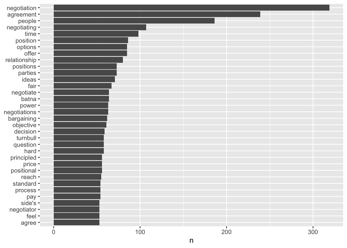

A Wordcloud?

# Make the wordcloud
tidy_book %>%
   count(word) %>%
   with(wordcloud(word, n, max.words = 100))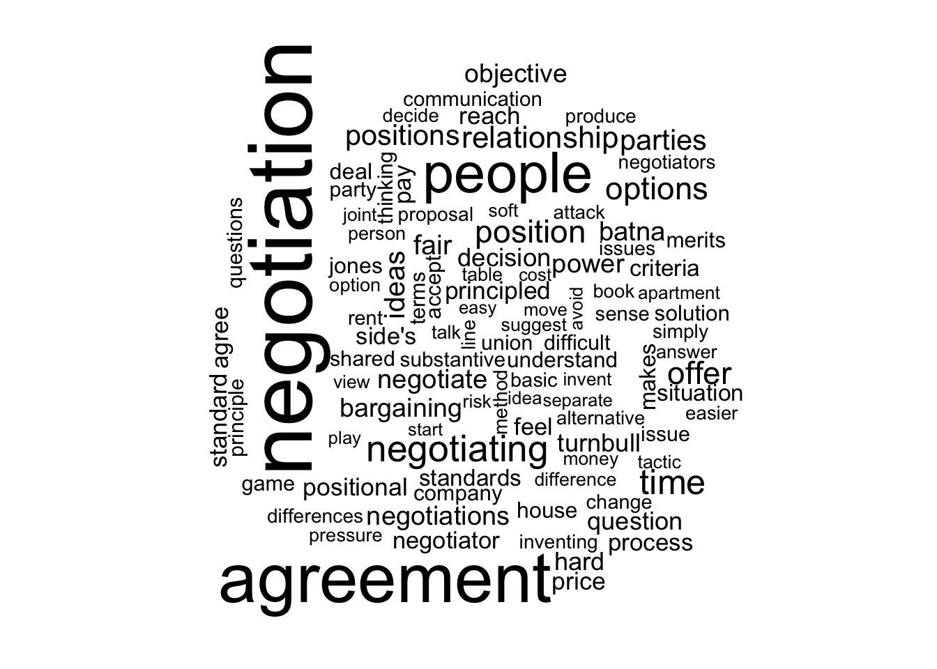

# Stems in lieu of words

Networks of Words

# Networks of words
library(igraph)
library(ggraph)
library(widyr)
count_bigrams <- function(dataset) {
  dataset %>%
    unnest_tokens(bigram, text, token = "ngrams", n = 2) %>%
    separate(bigram, c("word1", "word2"), sep = " ") %>%
    filter(!word1 %in% stop_words$word,
           !word2 %in% stop_words$word) %>%
    count(word1, word2, sort = TRUE)
}
word_cooccurences <- count_bigrams(Getting.To.Yes.TDF)
set.seed(2016)
word_cooccurences %>%
  filter(n >= 10) %>%
  graph_from_data_frame() %>%
  ggraph(layout = "fr") +
  geom_edge_link(aes(edge_alpha = n, edge_width = n)) +
  geom_node_point(color = "plum4", size = 5) +
  geom_node_text(aes(label = name), vjust = 1.8) +
  ggtitle(expression(paste("Word Network in", 
                           italic("Getting to Yes")))) +
  theme_void()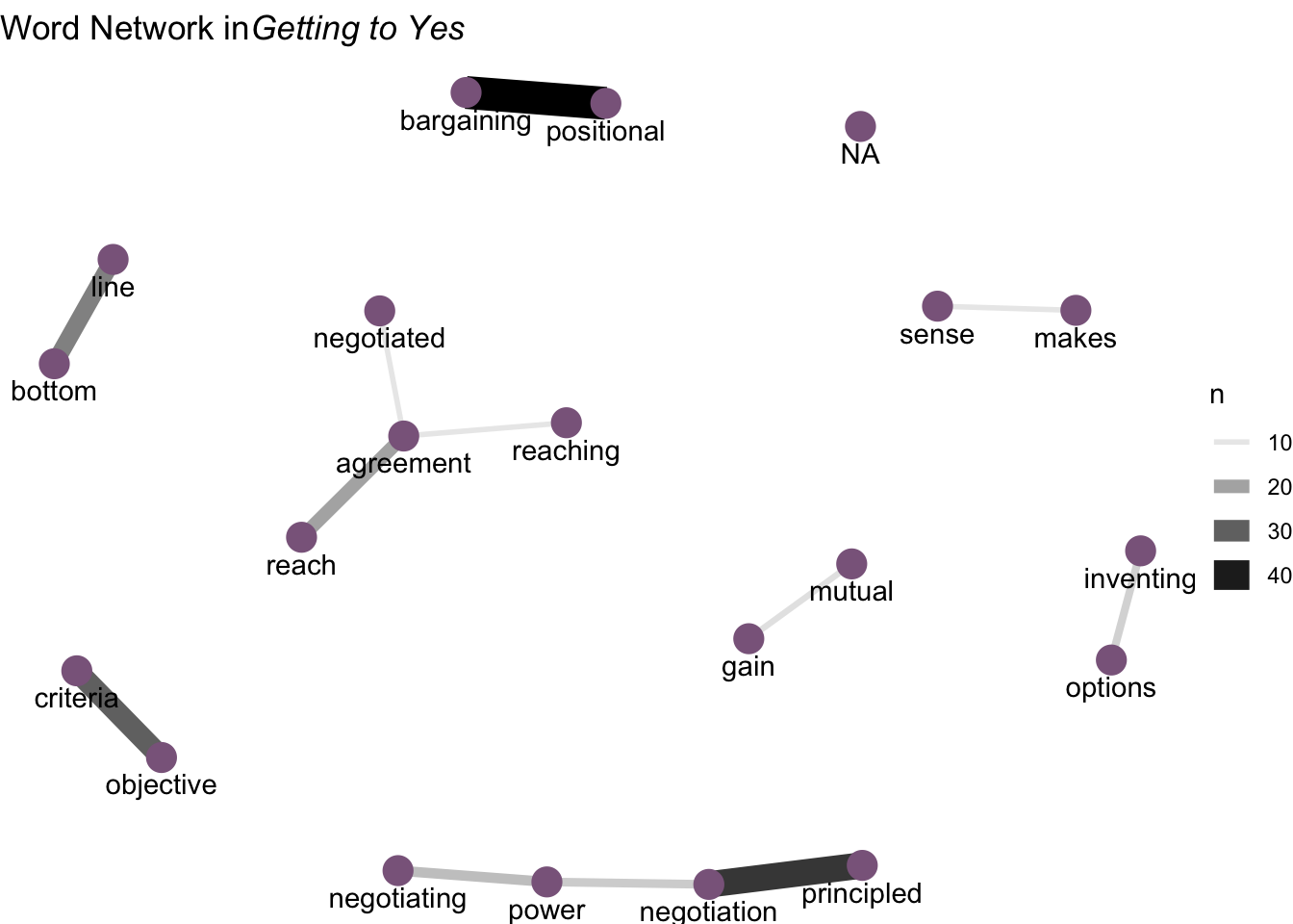

Other ways to plot them.

## More complicated breaks: pairs
GTY.PM <- Getting.To.Yes.TDF %>% 
  unnest_tokens(ngram, text, token = "ngrams", n = 2)
bigrams_separated <- GTY.PM %>%
  separate(ngram, c("word1", "word2"), sep = " ")

bigrams_filtered <- bigrams_separated %>%
  filter(!word1 %in% stop_words$word) %>%
  filter(!word2 %in% stop_words$word)

# new bigram counts:
bigram_counts <- bigrams_filtered %>% 
  count(word1, word2, sort = TRUE)

bigrams_united <- bigrams_filtered %>%
  unite(bigram, word1, word2, sep = " ")

my.df <- data.frame(table(bigrams_united$bigram))
my.df <- my.df[order(my.df$Freq, decreasing=TRUE),]
my.df <- my.df[c(2:100),]
head(my.df)

##                        Var1 Freq
## 2727  positional bargaining   44
## 2841 principled negotiation   36
## 2398     objective criteria   30
## 451             bottom line   25
## 3014        reach agreement   20
## 2264      negotiating power   16

bigram_counts

## # A tibble: 4,089 × 3
##    word1       word2           n
##    <chr>       <chr>       <int>
##  1 <NA>        <NA>          215
##  2 positional  bargaining     44
##  3 principled  negotiation    36
##  4 objective   criteria       30
##  5 bottom      line           25
##  6 reach       agreement      20
##  7 negotiating power          16
##  8 negotiation power          14
##  9 inventing   options        13
## 10 mutual      gain           11
## # … with 4,079 more rows

library(wordcloud2)
wordcloud2(my.df, color="random-light", backgroundColor = "black", size = 0.4)