Black Boxes: A Gender Gap Example
Variance in the Outcome: The Black Box
Regression models engage an exercise in variance accounting. How much of the outcome is explained by the inputs, individually (slope divided by standard error is t) and collectively (Average explained/Average unexplained with averaging over degrees of freedom is F). This, of course, assumes normal errors. This document provides a function for making use of the black box. Just as in common parlance, a black box is the unexplained. Let’s take an example.
options(scipen=10)
OregonSalaries <- structure(list(Obs = 1:32, Salary = c(41514.38701, 40964.06985,
39170.19178, 37936.57206, 33981.77752, 36077.27107, 39174.05733,
39037.372, 29131.74865, 36200.44592, 38561.3987, 33247.92306,
33609.4874, 33669.22275, 37805.83017, 35846.13454, 47342.65909,
46382.3851, 45812.91029, 46409.65664, 43796.05285, 43124.02135,
49443.81792, 44805.79217, 44440.32001, 46679.59218, 47337.09786,
47298.72531, 41461.0474, 43598.293, 43431.18499, 49266.41189),
    Gender = structure(c(1L, 1L, 1L, 1L, 1L, 1L, 1L, 1L, 1L,
    1L, 1L, 1L, 1L, 1L, 1L, 1L, 2L, 2L, 2L, 2L, 2L, 2L, 2L, 2L,
    2L, 2L, 2L, 2L, 2L, 2L, 2L, 2L), .Label = c("Female", "Male"
    ), class = "factor")), .Names = c("Obs", "Salary", "Gender"
), class = "data.frame", row.names = c(NA, -32L))
black.box.maker <- function(mod1) {
            d1 <- dim(mod1$model)[[1]]
            sumsq1 <- var(mod1$model[,1], na.rm=TRUE)*(d1-1)
            rt1 <- sqrt(sumsq1)
            sumsq2 <- var(mod1$fitted.values, na.rm=TRUE)*(d1-1)
            rsquare <- round(sumsq2/sumsq1, digits=4)
            rt2 <- sqrt(sumsq2)
            plot(x=NA, y=NA, xlim=c(0,rt1), ylim=c(0,rt1), main=paste("R-squared:",rsquare), xlab="", ylab="", bty="n", cex=0.5)
            polygon(x=c(0,0,rt1,rt1), y=c(0,rt1,rt1,0), col="black")
            polygon(x=c(0,0,rt2,rt2), y=c(0,rt2,rt2,0), col="green")
            }
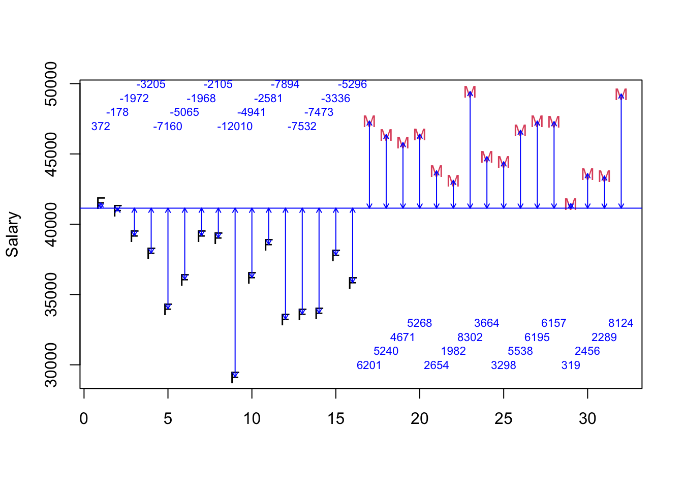
OregonSalaries contains 32 observations: 16 males and 16 females. The mean of all salaries is 41142.433; let me put that in a plot in blue. Represented in equation form, we have:
\[ Salary_{i} = \alpha + \epsilon_{i} \]
I will use \(\alpha\) in lieu of \(\mu\) because this is the most common method for demarcating an intercept, a recurring concept for regression models, but the above says that the \(i^{th}\) person’s salary is some average salary \(\alpha\) [or perhaps \(\mu\) to maintain conceptual continuity] plus some idiosyncratic remainder or residual salary for individual \(i\) denoted by \(\epsilon_{i}\).
The total sum of squares can be represented as the sum of all the squared distances to the blue line; each vertical distance is demarcated with an arrow below in blue. By definition, the vertical distances would/will sum to zero. The distance from the point to the line is also shown in blue; that is the residual salary. It shows how far that individual’s salary is from the overall average. The total sum of squares: the total area of the black box in the original metric (squared dollars) is: 892955385. The length of each side is the square root of that area, e.g. 892955384.31 in dollars.
ORSalScale <- scale(OregonSalaries$Salary, scale=FALSE)
plot(y=OregonSalaries$Salary, x=c(1:32), ylab="Salary", col=as.factor(OregonSalaries$Gender), xlab="", pch=c(rep("F",16),rep("M",16)))
abline(h=mean(OregonSalaries$Salary), col="blue")
arrows(x0=c(1:32), x1=c(1:32), y1=OregonSalaries$Salary,y0=mean(OregonSalaries$Salary), col="blue", code=3, length=0.05)
text(x=seq(1,16), y=rep(c(47000,48000,49000,50000),4), labels = paste(ceiling(ORSalScale[c(1:16)])), cex=0.7, col="blue")
text(x=c(17:32), y=rep(c(30000,31000,32000,33000),4), labels = paste(ceiling(ORSalScale[c(17:32)])), cex=0.7, col="blue")
Invoking the Function
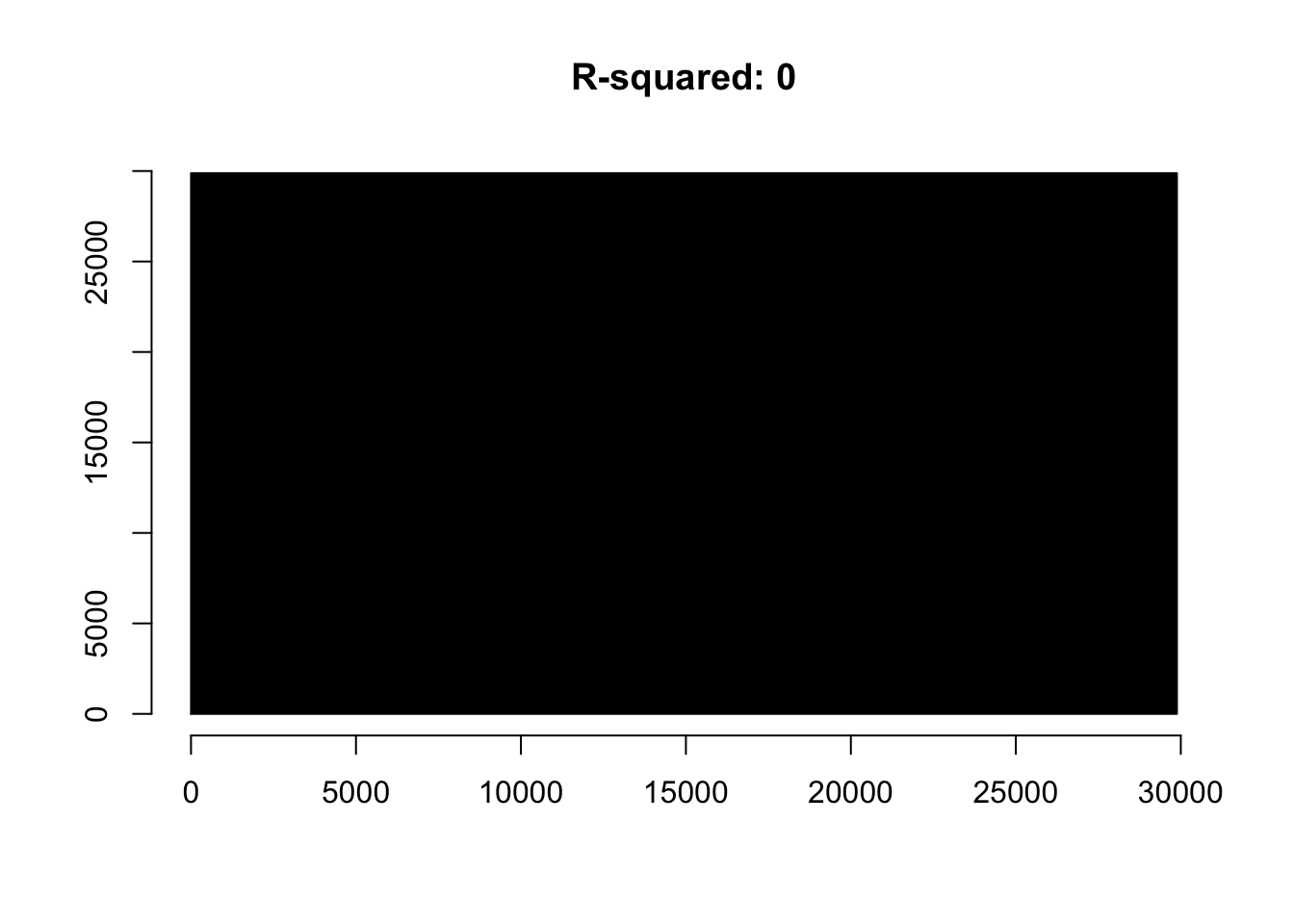
To represent the black box,let me draw it. The length of each side will be the square root of the black box; our total sum of squares is just under 900 million squared dollars so each side will be approximately 30000 dollars. The box appears below.
mod1 <- lm(Salary~1, data=OregonSalaries)
black.box.maker(mod1)
A Regression Model
I want to compare the constant mean for both groups that we labeled to be \(\alpha\) with an alternative that includes some non-zero [probably positive given ubiquitous evidence of gender gaps in compensation] difference between the two averages – a difference in averages. First, a regression model. I will estimate the following regression:
\[ Salary_{i} = \alpha + \beta_{1}*Gender_{i} + \epsilon_{i} \]
What does the regression imply? That salary for each individual \(i\) is a function of a constant and gender. Given the way that R works, \(\alpha\) will represent the average for females and \(\beta\) will represent the difference between male and female average salaries. The \(\epsilon\) will capture the difference between the individual’s salary and the average of their group (the mean of males or females).
A New Residual Sum of Squares
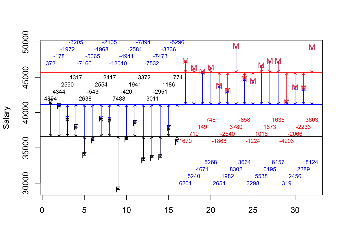
The picture will now have a red line and a black line and the residual/leftover/unexplained salary is now the difference between the point and the respective vertical line (red arrows or black arrows). What is the relationship between the datum and the group mean? The answer is shown in black/red.
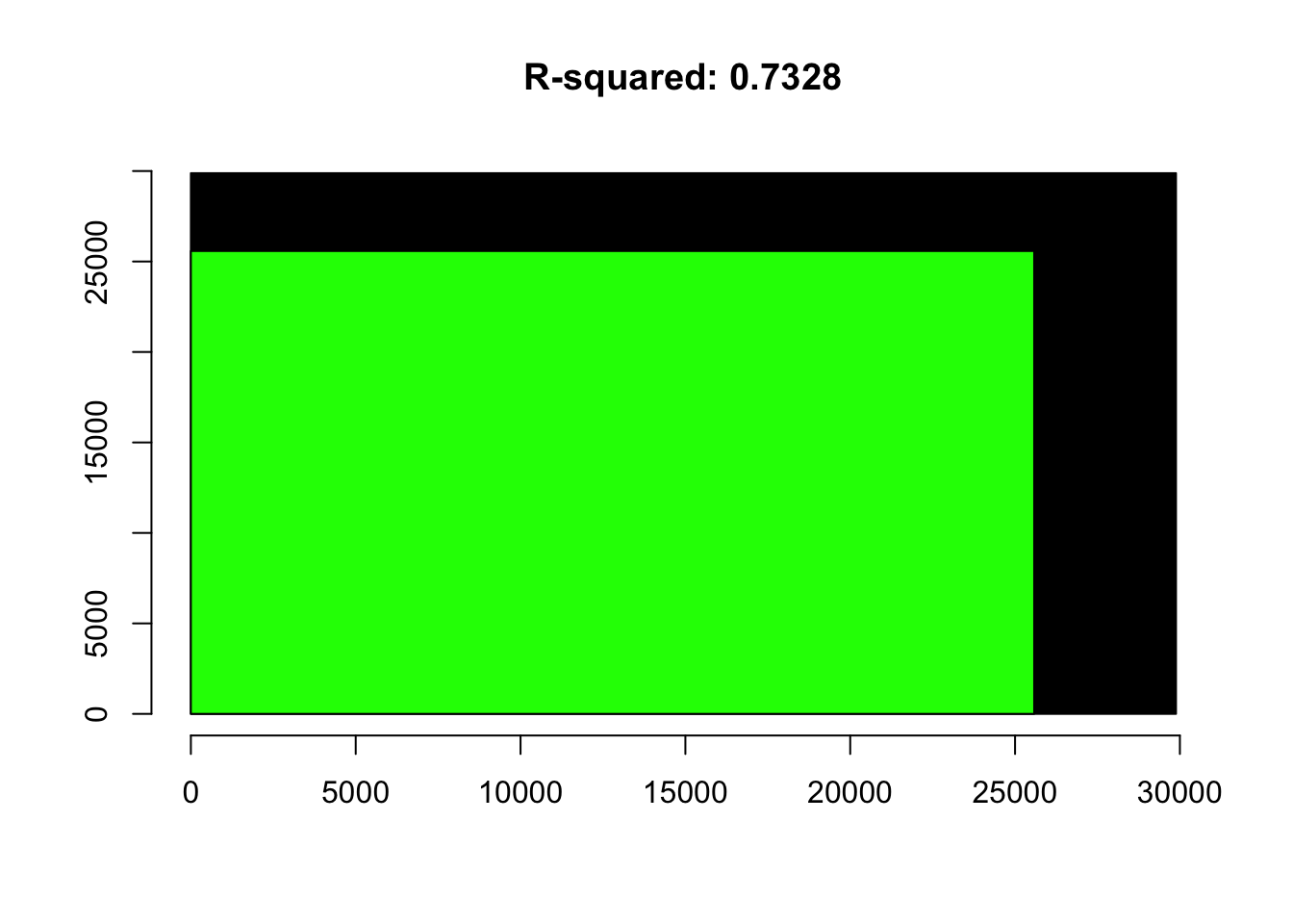
The sum of the remaining squared vertical distances is 238621277 is obtained by squaring the each black/red number. The amount explained by gender is the difference between each blue and the respective black/red number. It is important to notice that the highest paid females and the lowest paid males may have more residual salary given two averages but the different averages, overall, lead to far less residual salary than a single average for all salaries.
resids <- residuals(lm(Salary~Gender, data=OregonSalaries))
plot(y=OregonSalaries$Salary, x=c(1:32), ylab="Salary", col=as.factor(OregonSalaries$Gender), xlab="", pch=c(rep("F",16),rep("M",16)))
abline(h=mean(OregonSalaries$Salary), col="blue")
abline(h=mean(subset(OregonSalaries, Gender=="Female")$Salary, na.rm=T), col="black")
abline(h=mean(subset(OregonSalaries, Gender=="Male")$Salary, na.rm=T), col="red")
arrows(x0=c(1:32), x1=c(1:32), y1=OregonSalaries$Salary,y0=mean(OregonSalaries$Salary), col="blue", code=3, length=0.05)
arrows(x0=c(1:16), x1=c(1:16), y1=OregonSalaries$Salary[c(1:16)],y0=mean(subset(OregonSalaries, Gender=="Female")$Salary, na.rm=T), col="black", code=3, length=0.05)
arrows(x0=c(17:32), x1=c(17:32), y1=OregonSalaries$Salary[c(17:32)],y0=mean(subset(OregonSalaries, Gender=="Male")$Salary, na.rm=T), col="red", code=3, length=0.05)
text(x=seq(1,16), y=rep(c(47000,48000,49000,50000),4), labels = paste(ceiling(ORSalScale[c(1:16)])), cex=0.7, col="blue")
text(x=c(17:32), y=rep(c(30000,31000,32000,33000),4), labels = paste(ceiling(ORSalScale[c(17:32)])), cex=0.7, col="blue")
text(x=seq(1,16), y=rep(c(42000,43000,44000,45000),4), labels = paste(ceiling(resids[c(1:16)])), cex=0.7, col="black")
text(x=c(17:32), y=rep(c(36000,37000,38000,39000),4), labels = paste(ceiling(resids[c(17:32)])), cex=0.7, col="red")
The details of the regression estimates and the analysis of variance – the sums of squares – completes the rendering.
mod2 <- lm(Salary~Gender, data=OregonSalaries)
black.box.maker(mod2)
summary(mod1)##
## Call:
## lm(formula = Salary ~ 1, data = OregonSalaries)
##
## Residuals:
## Min 1Q Median 3Q Max
## -12010.7 -3737.9 345.3 4812.8 8301.4
##
## Coefficients:
## Estimate Std. Error t value Pr(>|t|)
## (Intercept) 41142.4 948.8 43.36 <2e-16 ***
## ---
## Signif. codes: 0 '***' 0.001 '**' 0.01 '*' 0.05 '.' 0.1 ' ' 1
##
## Residual standard error: 5367 on 31 degrees of freedomconfint(mod2)## 2.5 % 97.5 %
## (Intercept) 35180.542 38060.44
## GenderMale 7007.482 11080.28anova(mod1,mod2)## Analysis of Variance Table
##
## Model 1: Salary ~ 1
## Model 2: Salary ~ Gender
## Res.Df RSS Df Sum of Sq F Pr(>F)
## 1 31 892955384
## 2 30 238621277 1 654334108 82.264 0.0000000004223 ***
## ---
## Signif. codes: 0 '***' 0.001 '**' 0.01 '*' 0.05 '.' 0.1 ' ' 1