fredr is very neat
FRED via fredr
The Federal Reserve Economic Database [FRED] is a wonderful public resource for data and the r api that connects to it is very easy to use for the things that I have previously needed. For example, one of my students was interested in commercial credit default data. I used the FRED search instructions from the following vignette to find that data. My first step was the vignette for using fredr. Some library lines give me tools.
library(fredr); library(purrr)
library(dplyr)
##
## Attaching package: 'dplyr'## The following objects are masked from 'package:stats':
##
## filter, lag## The following objects are masked from 'package:base':
##
## intersect, setdiff, setequal, unionlibrary(ggplot2)A student wanted to find data on charge-offs. fredr has a search capability. Let’s see what we can find.
ChargeOff <- fredr_series_search_text(
  search_text = "real estate charge offs",
  order_by = "popularity",
  sort_order = "desc")
ChargeOff %>% select(title)
## # A tibble: 24 x 1
## title
## <chr>
## 1 Charge-Off Rate on Commercial Real Estate Loans (Excluding Farmland), Booked…
## 2 Charge-Off Rate on Loans Secured by Real Estate, All Commercial Banks
## 3 Net Charge-Offs on All Loans and Leases, Secured by Real Estate, Commercial …
## 4 Charge-Off Rate on Commercial Real Estate Loans (Excluding Farmland), Booked…
## 5 Net Charge-Offs on All Loans and Leases, Secured by Real Estate, Single Fami…
## 6 Charge-Off Rate on Commercial Real Estate Loans (Excluding Farmland), Booked…
## 7 Charge-Off Rate on Commercial Real Estate Loans (Excluding Farmland), Booked…
## 8 Charge-Off Rate on Loans Secured by Real Estate, Banks Not Among the 100 Lar…
## 9 Charge-Off Rate on Loans Secured by Real Estate, All Commercial Banks
## 10 Net Charge-Offs on All Loans and Leases, Secured by Real Estate, All Commerc…
## # … with 14 more rowsWow, there is a rich array of data from that query. An even cooler feature is the ability to retrieve multiple at once in combination with the map_dfr command from the purrr library to make it tidy; that will go through the search results and stack the data that is returned [bind it together by rows]. These map commands are the tidy version of apply. In this case, binding the columns will likely fail because the times series are unlikely to be of the same length and that would create ragged columns. Better tidy from the start here.
library(stringr)
ChargeOff.Data <- map_dfr(ChargeOff$id, fredr) %>% left_join(ChargeOff, by=c("series_id" = "id"))
Just to finish one piece, let me show what these data look like for one series. Splitting the name into two parts gives us the title and subtitle but the split is inconsistent so the solution is not general.
ChargeOff.Short <- ChargeOff.Data %>% filter(series_id=="CORSREOBS")
SeriesTitle <- ChargeOff.Short[1,"title"] %>% str_split(., "[,]") %>% unlist()
ChargeOff.Short %>% ggplot(data = ., mapping = aes(x = date, y = value)) +
    geom_line() +
    labs(x = "Date", y = "Rate", title=SeriesTitle[[1]], subtitle = SeriesTitle[[2]] )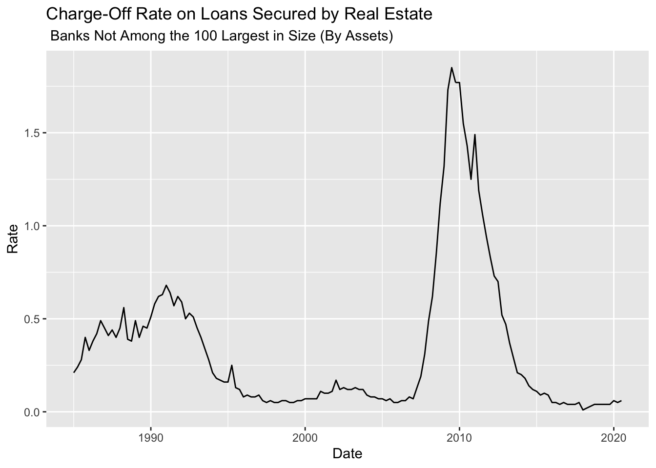
Counties and Mapping
When I was setting up fredr, I came across some data on subprime credit percentages. The data that I need for what I want to do is not obvious from the vignette and it turns out that this data is stored in a rather inconvenient fashion.
## # A tibble: 1 x 1
##   id
##   <chr>
## 1 EQFXSUBPRIME036061
The way that these are organized in FRED is going to make this a mess. The series_id actually contains data. Every data vector is stored as the series name and a FIPS code embdeded. The FIPS code is likely to be the last five characters/numbers. Fun. My other limitation is that I am only seeing 1000 of 3000+ counties. That’s a limit of the API. I am going to have to do this a bit differently. I am going to work backward. I have access to the full set of county fips codes so I think that I can build the dataset to query. Here goes.
library(readr)
CFIPS <- read_delim(url("https://github.com/robertwwalker/academic-mymod/raw/master/data/COUNTYFIPS.txt"), "\t", escape_double = FALSE, trim_ws = TRUE)
##
## ── Column specification ────────────────────────────────────────────────────────
## cols(
## FIPS = col_character(),
## Name = col_character(),
## State = col_character()
## )head(CFIPS)## # A tibble: 6 x 3
## FIPS Name State
## <chr> <chr> <chr>
## 1 01001 Autauga AL
## 2 01003 Baldwin AL
## 3 01005 Barbour AL
## 4 01007 Bibb AL
## 5 01009 Blount AL
## 6 01011 Bullock ALThat is all the FIPS codes that I will need. To create a new character vector for the data, it should just be a new column. From above, I know the names. Let me just concatenate the names to the FIPS code.
CFIPS$series_id <- as.character(paste0("EQFXSUBPRIME0",CFIPS$FIPS))Now for the moment of truth; I will only try this for Oregon.
SubPrime.OR <- CFIPS %>% filter(State=="OR") %>% select(series_id) %>% unlist() %>% map_dfr(., fredr)
SubPrime.OR <- left_join(SubPrime.OR, CFIPS, by="series_id")
SubPrime.OR %>% ggplot(aes(x=date, y=value, colour=series_id)) +
  geom_line() + theme(legend.position="none") + ggtitle("The Subprime Credit Rate Across Oregon Counties")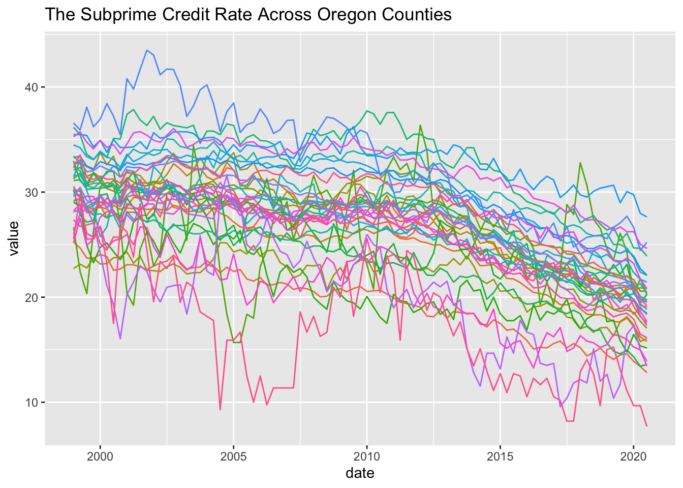
Now I have something to work with. Just to show what gganimate can do; I will animate that.
library(gganimate)
library(ggrepel)
library(tidyr)
SubPrime.OR %>% ggplot(aes(x=date, y=value, colour=series_id)) +
  geom_line() +
  geom_point(aes(group=series_id)) +
  geom_text_repel(aes(y = value, x = as.Date("2019-01-01"), label = Name), hjust = 1, nudge_x = 8) + theme(legend.position="none") + labs(title='The Subprime Credit Rate Across Oregon Counties: {frame_along}', y ="Subprime Rate") +
  transition_reveal(date)
## Warning: ggrepel: 26 unlabeled data points (too many overlaps). Consider
## increasing max.overlaps## Warning: ggrepel: 28 unlabeled data points (too many overlaps). Consider
## increasing max.overlaps## Warning: ggrepel: 24 unlabeled data points (too many overlaps). Consider
## increasing max.overlaps## Warning: ggrepel: 30 unlabeled data points (too many overlaps). Consider
## increasing max.overlaps
## Warning: ggrepel: 30 unlabeled data points (too many overlaps). Consider
## increasing max.overlaps## Warning: ggrepel: 29 unlabeled data points (too many overlaps). Consider
## increasing max.overlaps## Warning: ggrepel: 26 unlabeled data points (too many overlaps). Consider
## increasing max.overlaps## Warning: ggrepel: 25 unlabeled data points (too many overlaps). Consider
## increasing max.overlaps## Warning: ggrepel: 28 unlabeled data points (too many overlaps). Consider
## increasing max.overlaps## Warning: ggrepel: 25 unlabeled data points (too many overlaps). Consider
## increasing max.overlaps## Warning: ggrepel: 23 unlabeled data points (too many overlaps). Consider
## increasing max.overlaps## Warning: ggrepel: 27 unlabeled data points (too many overlaps). Consider
## increasing max.overlaps## Warning: ggrepel: 26 unlabeled data points (too many overlaps). Consider
## increasing max.overlaps
## Warning: ggrepel: 26 unlabeled data points (too many overlaps). Consider
## increasing max.overlaps
## Warning: ggrepel: 24 unlabeled data points (too many overlaps). Consider
## increasing max.overlaps
## Warning: ggrepel: 24 unlabeled data points (too many overlaps). Consider
## increasing max.overlaps
## Warning: ggrepel: 23 unlabeled data points (too many overlaps). Consider
## increasing max.overlaps
## Warning: ggrepel: 23 unlabeled data points (too many overlaps). Consider
## increasing max.overlaps
## Warning: ggrepel: 23 unlabeled data points (too many overlaps). Consider
## increasing max.overlaps## Warning: ggrepel: 22 unlabeled data points (too many overlaps). Consider
## increasing max.overlaps## Warning: ggrepel: 25 unlabeled data points (too many overlaps). Consider
## increasing max.overlaps
## Warning: ggrepel: 25 unlabeled data points (too many overlaps). Consider
## increasing max.overlaps## Warning: ggrepel: 26 unlabeled data points (too many overlaps). Consider
## increasing max.overlaps## Warning: ggrepel: 25 unlabeled data points (too many overlaps). Consider
## increasing max.overlaps## Warning: ggrepel: 22 unlabeled data points (too many overlaps). Consider
## increasing max.overlaps## Warning: ggrepel: 26 unlabeled data points (too many overlaps). Consider
## increasing max.overlaps## Warning: ggrepel: 24 unlabeled data points (too many overlaps). Consider
## increasing max.overlaps
## Warning: ggrepel: 24 unlabeled data points (too many overlaps). Consider
## increasing max.overlaps
## Warning: ggrepel: 24 unlabeled data points (too many overlaps). Consider
## increasing max.overlaps## Warning: ggrepel: 26 unlabeled data points (too many overlaps). Consider
## increasing max.overlaps## Warning: ggrepel: 24 unlabeled data points (too many overlaps). Consider
## increasing max.overlaps## Warning: ggrepel: 25 unlabeled data points (too many overlaps). Consider
## increasing max.overlaps
## Warning: ggrepel: 25 unlabeled data points (too many overlaps). Consider
## increasing max.overlaps## Warning: ggrepel: 26 unlabeled data points (too many overlaps). Consider
## increasing max.overlaps
## Warning: ggrepel: 26 unlabeled data points (too many overlaps). Consider
## increasing max.overlaps
## Warning: ggrepel: 26 unlabeled data points (too many overlaps). Consider
## increasing max.overlaps
## Warning: ggrepel: 26 unlabeled data points (too many overlaps). Consider
## increasing max.overlaps## Warning: ggrepel: 28 unlabeled data points (too many overlaps). Consider
## increasing max.overlaps## Warning: ggrepel: 27 unlabeled data points (too many overlaps). Consider
## increasing max.overlaps## Warning: ggrepel: 26 unlabeled data points (too many overlaps). Consider
## increasing max.overlaps## Warning: ggrepel: 21 unlabeled data points (too many overlaps). Consider
## increasing max.overlaps## Warning: ggrepel: 20 unlabeled data points (too many overlaps). Consider
## increasing max.overlaps
## Warning: ggrepel: 20 unlabeled data points (too many overlaps). Consider
## increasing max.overlaps## Warning: ggrepel: 19 unlabeled data points (too many overlaps). Consider
## increasing max.overlaps
## Warning: ggrepel: 19 unlabeled data points (too many overlaps). Consider
## increasing max.overlaps## Warning: ggrepel: 21 unlabeled data points (too many overlaps). Consider
## increasing max.overlaps## Warning: ggrepel: 20 unlabeled data points (too many overlaps). Consider
## increasing max.overlaps## Warning: ggrepel: 24 unlabeled data points (too many overlaps). Consider
## increasing max.overlaps## Warning: ggrepel: 20 unlabeled data points (too many overlaps). Consider
## increasing max.overlaps## Warning: ggrepel: 24 unlabeled data points (too many overlaps). Consider
## increasing max.overlaps## Warning: ggrepel: 25 unlabeled data points (too many overlaps). Consider
## increasing max.overlaps## Warning: ggrepel: 24 unlabeled data points (too many overlaps). Consider
## increasing max.overlaps
## Warning: ggrepel: 24 unlabeled data points (too many overlaps). Consider
## increasing max.overlaps
## Warning: ggrepel: 24 unlabeled data points (too many overlaps). Consider
## increasing max.overlaps## Warning: ggrepel: 27 unlabeled data points (too many overlaps). Consider
## increasing max.overlaps## Warning: ggrepel: 24 unlabeled data points (too many overlaps). Consider
## increasing max.overlaps## Warning: ggrepel: 23 unlabeled data points (too many overlaps). Consider
## increasing max.overlaps## Warning: ggrepel: 25 unlabeled data points (too many overlaps). Consider
## increasing max.overlaps
## Warning: ggrepel: 25 unlabeled data points (too many overlaps). Consider
## increasing max.overlaps
## Warning: ggrepel: 25 unlabeled data points (too many overlaps). Consider
## increasing max.overlaps
## Warning: ggrepel: 27 unlabeled data points (too many overlaps). Consider
## increasing max.overlaps
## Warning: ggrepel: 27 unlabeled data points (too many overlaps). Consider
## increasing max.overlaps
## Warning: ggrepel: 27 unlabeled data points (too many overlaps). Consider
## increasing max.overlaps## Warning: ggrepel: 25 unlabeled data points (too many overlaps). Consider
## increasing max.overlaps## Warning: ggrepel: 27 unlabeled data points (too many overlaps). Consider
## increasing max.overlaps## Warning: ggrepel: 24 unlabeled data points (too many overlaps). Consider
## increasing max.overlaps## Warning: ggrepel: 25 unlabeled data points (too many overlaps). Consider
## increasing max.overlaps
## Warning: ggrepel: 25 unlabeled data points (too many overlaps). Consider
## increasing max.overlaps
## Warning: ggrepel: 25 unlabeled data points (too many overlaps). Consider
## increasing max.overlaps## Warning: ggrepel: 24 unlabeled data points (too many overlaps). Consider
## increasing max.overlaps
## Warning: ggrepel: 24 unlabeled data points (too many overlaps). Consider
## increasing max.overlaps## Warning: ggrepel: 22 unlabeled data points (too many overlaps). Consider
## increasing max.overlaps## Warning: ggrepel: 24 unlabeled data points (too many overlaps). Consider
## increasing max.overlaps## Warning: ggrepel: 22 unlabeled data points (too many overlaps). Consider
## increasing max.overlaps## Warning: ggrepel: 25 unlabeled data points (too many overlaps). Consider
## increasing max.overlaps## Warning: ggrepel: 23 unlabeled data points (too many overlaps). Consider
## increasing max.overlaps## Warning: ggrepel: 26 unlabeled data points (too many overlaps). Consider
## increasing max.overlaps## Warning: ggrepel: 24 unlabeled data points (too many overlaps). Consider
## increasing max.overlaps## Warning: ggrepel: 23 unlabeled data points (too many overlaps). Consider
## increasing max.overlaps
## Warning: ggrepel: 23 unlabeled data points (too many overlaps). Consider
## increasing max.overlaps
## Warning: ggrepel: 23 unlabeled data points (too many overlaps). Consider
## increasing max.overlaps## Warning: ggrepel: 24 unlabeled data points (too many overlaps). Consider
## increasing max.overlaps
## Warning: ggrepel: 24 unlabeled data points (too many overlaps). Consider
## increasing max.overlaps## Warning: ggrepel: 25 unlabeled data points (too many overlaps). Consider
## increasing max.overlaps
## Warning: ggrepel: 25 unlabeled data points (too many overlaps). Consider
## increasing max.overlaps

## Warning: ggrepel: 25 unlabeled data points (too many overlaps). Consider
## increasing max.overlaps
## Warning: ggrepel: 25 unlabeled data points (too many overlaps). Consider
## increasing max.overlaps
## Warning: ggrepel: 24 unlabeled data points (too many overlaps). Consider
## increasing max.overlaps## Warning: ggrepel: 26 unlabeled data points (too many overlaps). Consider
## increasing max.overlaps## Warning: ggrepel: 25 unlabeled data points (too many overlaps). Consider
## increasing max.overlaps## Warning: ggrepel: 29 unlabeled data points (too many overlaps). Consider
## increasing max.overlaps## Warning: ggrepel: 27 unlabeled data points (too many overlaps). Consider
## increasing max.overlaps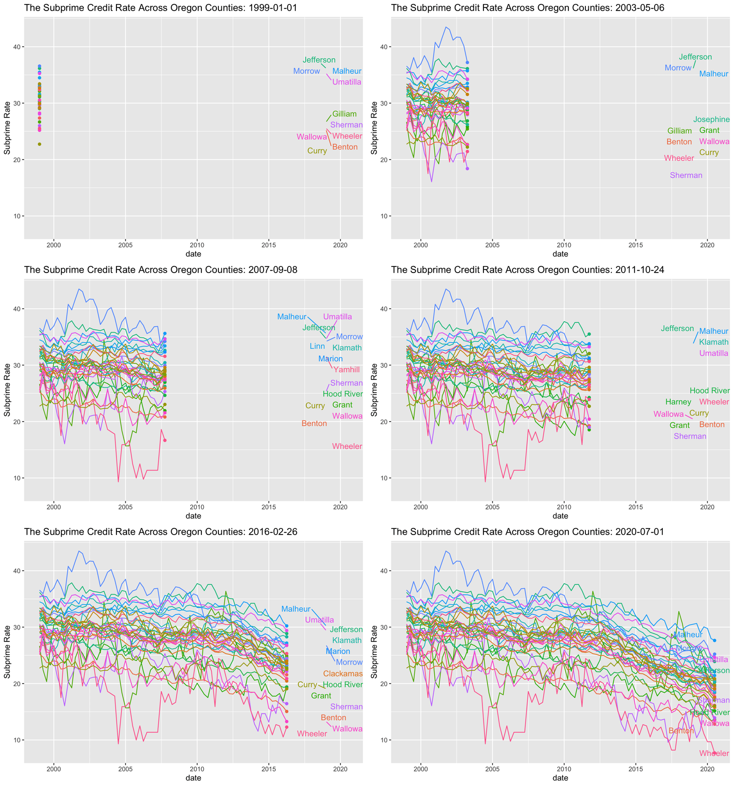
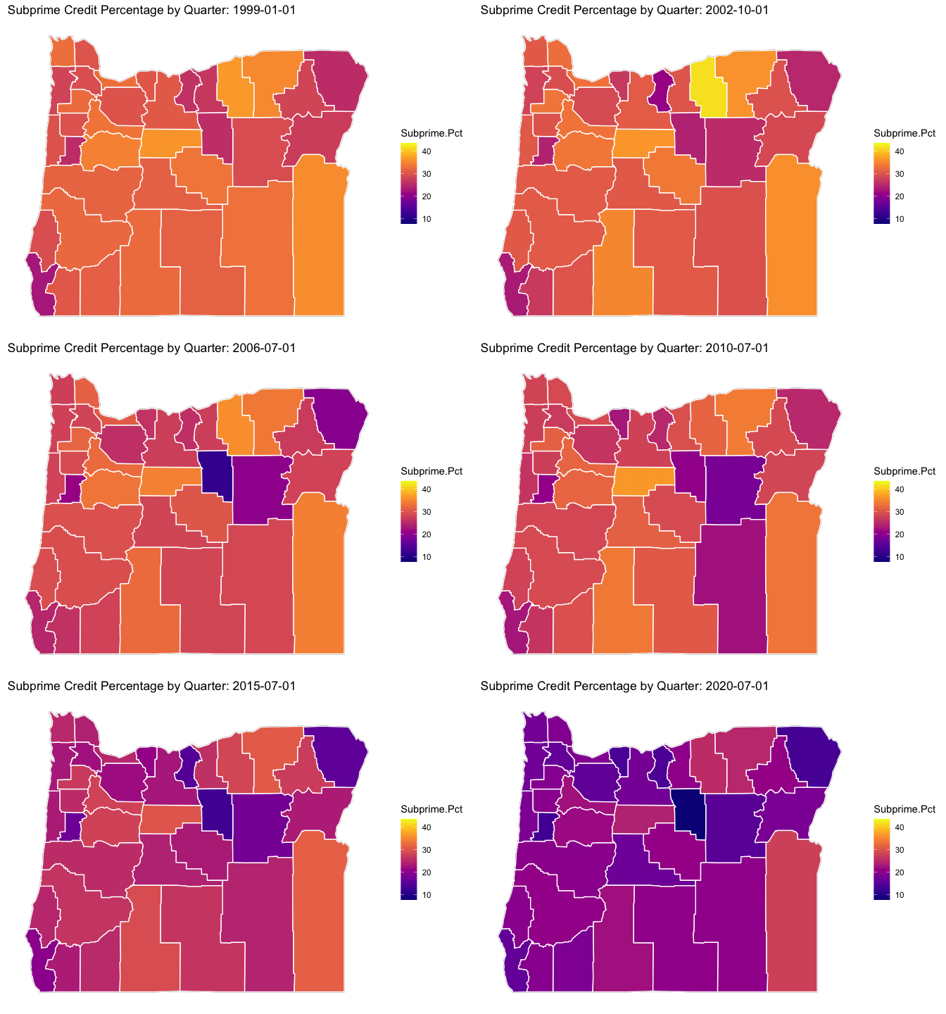
My goal here is to build an animation of the map of this. So here goes.
states <- map_data("state")
OR.df <- subset(states, region == "oregon")
OR_base <- ggplot(data = OR.df, mapping = aes(x = long, y = lat, group = group)) +
geom_polygon(color = "black", fill = "gray")+ theme_minimal()
OR_base + geom_point(aes(x=-123.0433, y=44.925167))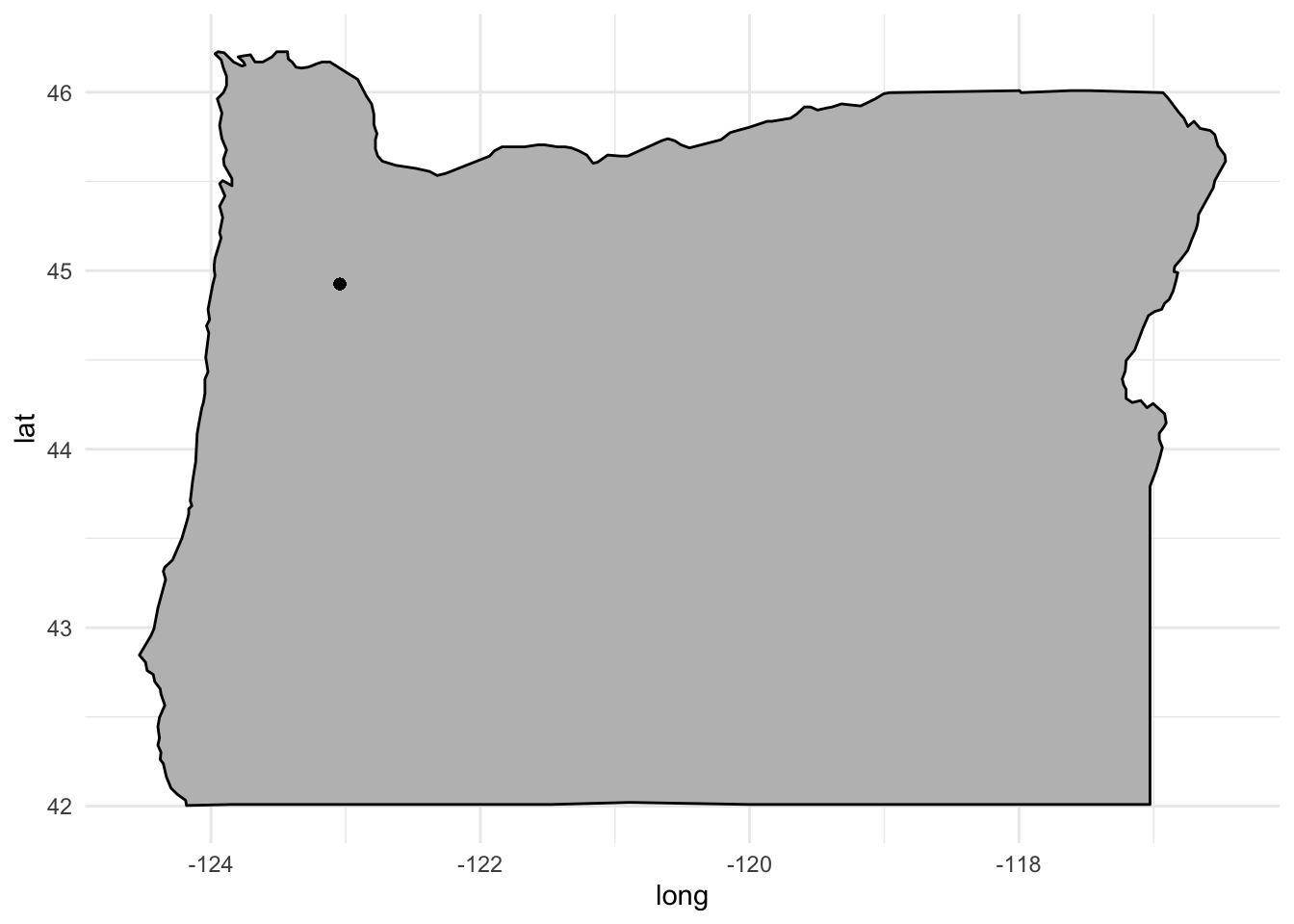
library(emoGG)
counties <- map_data("county")
OR.county <- subset(counties, region == "oregon")
OR.Map <- ggplot(data = OR.df, mapping = aes(x = long, y = lat, group = group)) +
    geom_polygon(color = "black", fill = "gray")+ theme_minimal()
OR_emoj <- OR_base +  add_emoji("1f352", x=-123.0433, y=44.925167, ysize=0.5)
OR_emoj
Now to build a first map to make sure that it works.
library(maps)##
## Attaching package: 'maps'## The following object is masked from 'package:purrr':
##
## mapcounty.fips$fips <- as.character(county.fips$fips)
SubPrime.M <- left_join(SubPrime.OR, county.fips, by=c("FIPS"="fips"))
SubPrime.M <- SubPrime.M %>% separate(., polyname, c("region","subregion"), sep=",")
SubPrime.M %>% filter(date=="1999-01-01") -> OneYear
OR.MD <- inner_join(OR.county, OneYear, by = "subregion")One of my favortite bits of code from I do not know where:
ditch_the_axes <- theme(
  axis.text = element_blank(),
  axis.line = element_blank(),
  axis.ticks = element_blank(),
  panel.border = element_blank(),
  panel.grid = element_blank(),
  axis.title = element_blank()
  )
Now to a single map.
Polt1 <- OR.Map +
      geom_polygon(data = OR.MD, aes(fill = value), color="white") +
#      geom_polygon(color = "black", fill = NA) +
      theme_bw() +
      ditch_the_axes +
      ggtitle("Subprime Credit Percentages by County")
Polt1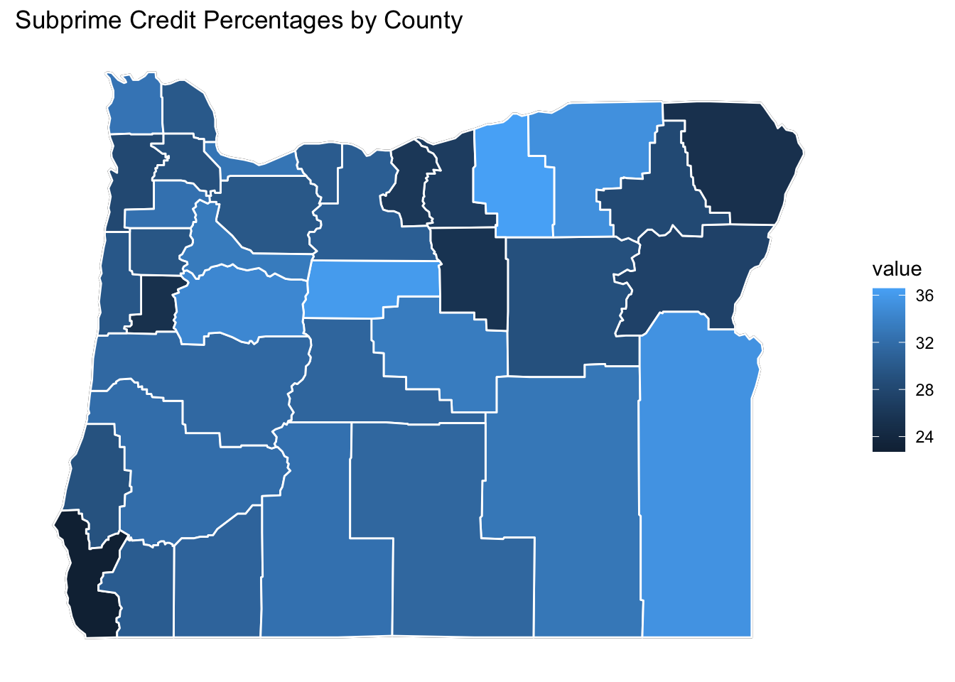
Now for the general case. Same merge but with all the data.
OR.MD2 <- left_join(SubPrime.M, OR.county, by = "subregion")
OR.MD2 <- OR.MD2 %>% mutate(Subprime.Pct = value)
Here goes.
library(viridis)## Loading required package: viridisLite# ggplot(data = OR.MD2, mapping = aes(x = long, y = lat, group = group)) +
p <- OR.Map +
geom_polygon(data=OR.MD2, aes(x = long, y = lat, group = subregion, fill = Subprime.Pct), color="white") +
viridis::scale_fill_viridis(option="C") +
ditch_the_axes +
labs(title = 'Subprime Credit Percentage by Quarter: {closest_state}') +
transition_states(date, transition_length = 3, state_length = 3)
animate(p, nframes = 300)