nflscrapR is amazing
Scraping NFL data
Note: An original version of this post had issues induced by overtime games. There is a better way to handle all of this that I learned from a brief analysis of a tie game between Cleveland and Pittsburgh in Week One.
The nflscrapR package is designed to make data on NFL games more easily available. To install the package, we need to grab it from github. The package provides play by play data available for entire NFL seasons. Numerous fascinating applications of this data have come out of the Sloan Conference and other places that do cutting edge sports analytics.
devtools::install_github(repo = "maksimhorowitz/nflscrapR")The github page for nflscrapR is quite informative.
Getting Some Data
Following the guide to the package on GitHub, let me try their example. It works, but I will save off the data to github to avoid spamming the host.
library(nflscrapR)
all_2018_games <- scrape_game_ids(2018) # Default is regular season
Gives me a list of all games. I saved them to an .rds file and stored them on Gitub. To make it browsable, I will use kable and the like.
library(tidyverse)
library(nflscrapR)
library(RCurl)
library(kableExtra)
library(gganimate)
library(ggrepel)
library(ggthemes)
library(RColorBrewer)
library(janitor)
all_2018_games <-readRDS(url("https://github.com/robertwwalker/academic-mymod/raw/master/data/NFLGames2018.rds"))
all_2018_games %>%  kable()  %>%
  kable_styling() %>%
scroll_box(width = "100%", height = "300px")That’s all the regular season games in the 2018 season. They suggest that it is straightforward to grab an entire season of play by play data.
full_season_2018 <- scrape_season_play_by_play(2018, "reg")
saveRDS(full_season_2018, file="../../../data/2018NFLSeason.rds")
That gets the data though it took over an hour to acquire it all and it threw two error messages. I do not yet know if they are conseequential. My goal here is to use this package and the ability to plot the win probability charts to try to summarise an entire cowboys season.
full_season_2018 <- readRDS(url("https://github.com/robertwwalker/academic-mymod/raw/master/data/2018NFLSeason.rds")) What can I do with it?
When I paid attention the NFL, I followed the Dallas Cowboys. Let’s isolate their data.
dal_season <- full_season_2018 %>% filter(home_team=="DAL" | away_team=="DAL")
dal_season %>%  head()
## # A tibble: 6 x 256
## play_id game_id home_team away_team posteam posteam_type defteam side_of_field
## <chr> <chr> <chr> <chr> <chr> <chr> <chr> <chr>
## 1 36 201809… CAR DAL DAL away CAR CAR
## 2 51 201809… CAR DAL DAL away CAR DAL
## 3 72 201809… CAR DAL DAL away CAR DAL
## 4 107 201809… CAR DAL DAL away CAR DAL
## 5 128 201809… CAR DAL DAL away CAR DAL
## 6 151 201809… CAR DAL DAL away CAR DAL
## # … with 248 more variables: yardline_100 <dbl>, game_date <date>,
## # quarter_seconds_remaining <dbl>, half_seconds_remaining <dbl>,
## # game_seconds_remaining <dbl>, game_half <chr>, quarter_end <dbl>,
## # drive <int>, sp <dbl>, qtr <dbl>, down <fct>, goal_to_go <dbl>, time <chr>,
## # yrdln <chr>, ydstogo <dbl>, ydsnet <dbl>, desc <chr>, play_type <chr>,
## # yards_gained <dbl>, shotgun <dbl>, no_huddle <dbl>, qb_dropback <dbl>,
## # qb_kneel <dbl>, qb_spike <dbl>, qb_scramble <dbl>, pass_length <chr>,
## # pass_location <chr>, air_yards <dbl>, yards_after_catch <dbl>,
## # run_location <chr>, run_gap <chr>, field_goal_result <chr>,
## # kick_distance <dbl>, extra_point_result <chr>, two_point_conv_result <chr>,
## # home_timeouts_remaining <dbl>, away_timeouts_remaining <dbl>,
## # timeout <dbl>, timeout_team <chr>, td_team <chr>,
## # posteam_timeouts_remaining <dbl>, defteam_timeouts_remaining <dbl>,
## # total_home_score <dbl>, total_away_score <dbl>, posteam_score <dbl>,
## # defteam_score <dbl>, score_differential <dbl>, posteam_score_post <dbl>,
## # defteam_score_post <dbl>, score_differential_post <dbl>,
## # no_score_prob <dbl>, opp_fg_prob <dbl>, opp_safety_prob <dbl>,
## # opp_td_prob <dbl>, fg_prob <dbl>, safety_prob <dbl>, td_prob <dbl>,
## # extra_point_prob <dbl>, two_point_conversion_prob <dbl>, ep <dbl>,
## # epa <dbl>, total_home_epa <dbl>, total_away_epa <dbl>,
## # total_home_rush_epa <dbl>, total_away_rush_epa <dbl>,
## # total_home_pass_epa <dbl>, total_away_pass_epa <dbl>, air_epa <dbl>,
## # yac_epa <dbl>, comp_air_epa <dbl>, comp_yac_epa <dbl>,
## # total_home_comp_air_epa <dbl>, total_away_comp_air_epa <dbl>,
## # total_home_comp_yac_epa <dbl>, total_away_comp_yac_epa <dbl>,
## # total_home_raw_air_epa <dbl>, total_away_raw_air_epa <dbl>,
## # total_home_raw_yac_epa <dbl>, total_away_raw_yac_epa <dbl>, wp <dbl>,
## # def_wp <dbl>, home_wp <dbl>, away_wp <dbl>, wpa <dbl>, home_wp_post <dbl>,
## # away_wp_post <dbl>, total_home_rush_wpa <dbl>, total_away_rush_wpa <dbl>,
## # total_home_pass_wpa <dbl>, total_away_pass_wpa <dbl>, air_wpa <dbl>,
## # yac_wpa <dbl>, comp_air_wpa <dbl>, comp_yac_wpa <dbl>,
## # total_home_comp_air_wpa <dbl>, total_away_comp_air_wpa <dbl>,
## # total_home_comp_yac_wpa <dbl>, total_away_comp_yac_wpa <dbl>,
## # total_home_raw_air_wpa <dbl>, total_away_raw_air_wpa <dbl>, …# kable() %>%
# kable_styling() %>%
# scroll_box(width = "100%", height = "200px")Dallas Season
Now I want to try and build a plot of all of Dallas Cowboys games for the season. Here are the steps. First, I am going to make a table that contains all of the names and colors for all of the game IDs. Even though I only need those for Dallas, building a shiny app for this would mean that I could select by teams above and make it extensible. At the end, I will only need those for Dallas so I will separate them off.
all_2018_games %>% select(home_team, home_score, away_team, away_score) %>% head()## home_team home_score away_team away_score
## 1 PHI 18 ATL 12
## 2 BAL 47 BUF 3
## 3 NYG 15 JAX 20
## 4 NO 40 TB 48
## 5 NE 27 HOU 20
## 6 MIN 24 SF 16Cool.
ntable <- all_2018_games %>% select(game_id, home_team, away_team)
ntableH <- ntable
ntableH <- ntableH %>% left_join(nflteams, by = c("home_team" = "abbr"))
names(ntableH) <- paste0("Home_",names(ntableH), sep="")
ntableH <- ntableH %>% rename(., game_id = Home_game_id, home_team = Home_home_team, away_team = Home_away_team)
ntableA <- ntable
ntableA <- ntableA %>% left_join(nflteams, by = c("away_team" = "abbr"))
names(ntableA) <- paste0("Away_",names(ntableA), sep="")
ntableA <- ntableA %>% rename(., game_id = Away_game_id, home_team = Away_home_team, away_team = Away_away_team)
My.NFL.Table <- ntableH %>% inner_join(ntableA)
## Joining, by = c("game_id", "home_team", "away_team")My.NFL.Table <- My.NFL.Table %>% left_join(all_2018_games)## Joining, by = c("game_id", "home_team", "away_team")Dallas.Table <- My.NFL.Table %>% filter(home_team=="DAL" | away_team=="DAL")
Dallas.Table %>% head()## game_id home_team away_team Home_team Home_primary Home_secondary
## 1 2018090910 CAR DAL Carolina Panthers #0085ca #000000
## 2 2018091613 DAL NYG Dallas Cowboys #002244 #b0b7bc
## 3 2018092312 SEA DAL Seattle Seahawks #002244 #69be28
## 4 2018093002 DAL DET Dallas Cowboys #002244 #b0b7bc
## 5 2018100712 HOU DAL Houston Texans #03202f #a71930
## 6 2018101410 DAL JAX Dallas Cowboys #002244 #b0b7bc
## Home_tertiary Home_quaternary Home_division Away_team Away_primary
## 1 #bfc0bf #0085ca NFC South Dallas Cowboys #002244
## 2 #acc0c6 #a5acaf NFC East New York Giants #0b2265
## 3 #a5acaf #001532 NFC West Dallas Cowboys #002244
## 4 #acc0c6 #a5acaf NFC East Detroit Lions #005a8b
## 5 #00071c #a30d2d AFC South Dallas Cowboys #002244
## 6 #acc0c6 #a5acaf NFC East Jacksonville Jaguars #000000
## Away_secondary Away_tertiary Away_quaternary Away_division type week season
## 1 #b0b7bc #acc0c6 #a5acaf NFC East reg 1 2018
## 2 #a71930 #a5acaf #012352 NFC East reg 2 2018
## 3 #b0b7bc #acc0c6 #a5acaf NFC East reg 3 2018
## 4 #b0b7bc #000000 #004e89 NFC North reg 4 2018
## 5 #b0b7bc #acc0c6 #a5acaf NFC East reg 5 2018
## 6 #006778 #9f792c #d7a22a AFC South reg 6 2018
## state_of_game
## 1 POST
## 2 POST
## 3 POST
## 4 POST
## 5 POST
## 6 POST
## game_url
## 1 http://www.nfl.com/liveupdate/game-center/2018090910/2018090910_gtd.json
## 2 http://www.nfl.com/liveupdate/game-center/2018091613/2018091613_gtd.json
## 3 http://www.nfl.com/liveupdate/game-center/2018092312/2018092312_gtd.json
## 4 http://www.nfl.com/liveupdate/game-center/2018093002/2018093002_gtd.json
## 5 http://www.nfl.com/liveupdate/game-center/2018100712/2018100712_gtd.json
## 6 http://www.nfl.com/liveupdate/game-center/2018101410/2018101410_gtd.json
## home_score away_score
## 1 16 8
## 2 20 13
## 3 24 13
## 4 26 24
## 5 19 16
## 6 40 7One nice little bit of data recovery here, the season schedule and Dallas’s result can be seen below.
Dallas.Table %>% select(game_id,Home_team,home_score, Away_team, away_score)## game_id Home_team home_score Away_team away_score
## 1 2018090910 Carolina Panthers 16 Dallas Cowboys 8
## 2 2018091613 Dallas Cowboys 20 New York Giants 13
## 3 2018092312 Seattle Seahawks 24 Dallas Cowboys 13
## 4 2018093002 Dallas Cowboys 26 Detroit Lions 24
## 5 2018100712 Houston Texans 19 Dallas Cowboys 16
## 6 2018101410 Dallas Cowboys 40 Jacksonville Jaguars 7
## 7 2018102110 Washington Redskins 20 Dallas Cowboys 17
## 8 2018110500 Dallas Cowboys 14 Tennessee Titans 28
## 9 2018111111 Philadelphia Eagles 20 Dallas Cowboys 27
## 10 2018111800 Atlanta Falcons 19 Dallas Cowboys 22
## 11 2018112201 Dallas Cowboys 31 Washington Redskins 23
## 12 2018112900 Dallas Cowboys 13 New Orleans Saints 10
## 13 2018120912 Dallas Cowboys 29 Philadelphia Eagles 23
## 14 2018121605 Indianapolis Colts 23 Dallas Cowboys 0
## 15 2018122306 Dallas Cowboys 27 Tampa Bay Buccaneers 20
## 16 2018123008 New York Giants 35 Dallas Cowboys 36Season Won-Loss Records
To derive a season won-loss record for each team, I need to first declare the outcome of each game using the scores and then summarise them over teams. I will also have to pass them on because they do not have this in the nflteams data in nflscrapR.
WLTabs <- all_2018_games %>% mutate(home_win = (home_score > away_score), away_win = (away_score > home_score)) %>% select(game_id, home_team, away_team, home_win, away_win) %>% gather("home_team", "away_team", key="HA", value="abbr")
WLTabs$Wins <- WLTabs$home_win
WLTabs[WLTabs$HA=="away_team","Wins"] <- WLTabs[WLTabs$HA=="away_team","away_win"]
WinsTab <- WLTabs %>% group_by(abbr) %>% summarise(Wins = sum(Wins==TRUE))
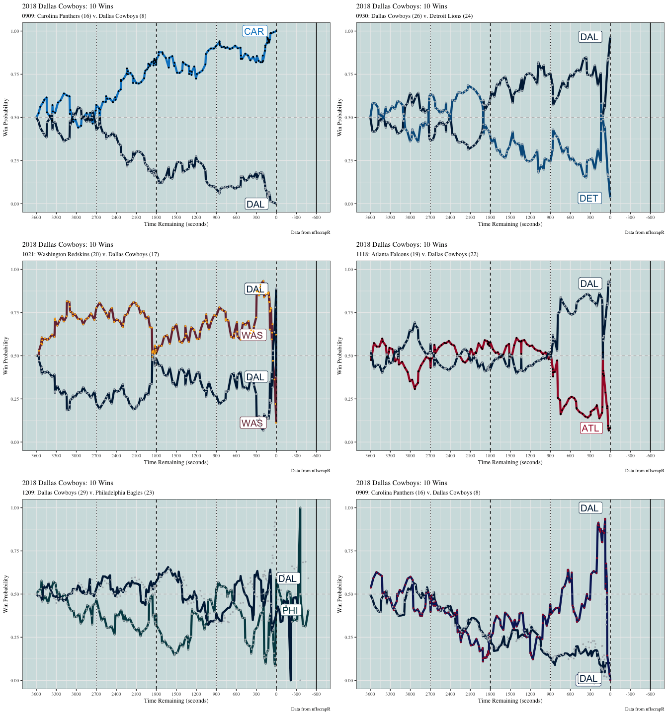
Now I want to put together a plot of a season. The way to make it modular is to choose a team and program the rest as a function with that as input. The hack that I undertook is recalibrating the time remaining to take account of the mess of overtime games.
season_animator <- function(teamName, data1=full_season_2018, data2=all_2018_games, nflteams = nflscrapR::nflteams) {
  # This creates the team color vector
  NFL.colors <- nflteams %>% select(primary)
  NFL.colors <- as.vector(NFL.colors$primary)
  names(NFL.colors) <- nflteams$abbr
  NFL.colorsS <- nflteams %>% select(secondary)
  NFL.colorsS <- as.vector(NFL.colorsS$secondary)
  names(NFL.colorsS) <- nflteams$abbr
  # Now create the title and wins
  WLTabs <- all_2018_games %>% mutate(home_win = (home_score > away_score), away_win = (away_score > home_score)) %>% select(game_id, home_team, away_team, home_win, away_win) %>% gather("home_team", "away_team", key="HA", value="abbr")
  WLTabs$Wins <- WLTabs$home_win
  WLTabs[WLTabs$HA=="away_team","Wins"] <- WLTabs[WLTabs$HA=="away_team","away_win"]
  WinsTab <- WLTabs %>% group_by(abbr) %>% summarise(Wins = sum(Wins==TRUE))
  My.Wins <- WinsTab %>% filter(abbr==teamName) %>% select(Wins) %>% as.integer()
  title.ST <- nflteams %>% filter(abbr==teamName) %>% select(team) %>% as.character()
  title.My <- paste0("2018 ",title.ST,": ",My.Wins," Wins")
  ntable <- all_2018_games %>% select(game_id, home_team, away_team)
  ntableH <- ntable
  ntableH <- ntableH %>% left_join(nflteams, by = c("home_team" = "abbr"))
  names(ntableH) <- paste0("Home_",names(ntableH), sep="")
  ntableH <- ntableH %>% rename(., game_id = Home_game_id, home_team = Home_home_team, away_team = Home_away_team)
  ntableA <- ntable
  ntableA <- ntableA %>% left_join(nflteams, by = c("away_team" = "abbr"))
  names(ntableA) <- paste0("Away_",names(ntableA), sep="")
  ntableA <- ntableA %>% rename(., game_id = Away_game_id, home_team = Away_home_team, away_team = Away_away_team)
  My.NFL.Table <- ntableH %>% inner_join(ntableA)
  My.NFL.Table <- My.NFL.Table %>% left_join(all_2018_games)
  # Select off the team dataset
  team_season <- full_season_2018 %>% filter(home_team==teamName | away_team==teamName)
  # Fix GSR
  team_season[team_season$game_half=="Overtime","game_seconds_remaining"] <- -1*(600 - team_season[team_season$game_half=="Overtime","game_seconds_remaining"])
  team_wp <- team_season %>%
    filter(!is.na(home_wp),!is.na(away_wp)) %>%
    unite(GIDGSR, game_seconds_remaining, game_id, sep=":")
  team_wp <- team_wp %>%
    dplyr::select(GIDGSR,
                  home_wp,
                  away_wp)  %>%
    gather(team, wpa, -GIDGSR) %>%
    separate(., GIDGSR, c("GSR", "game_id"), sep=":") %>%
    mutate(game_seconds_remaining = as.integer(GSR))
  team_plt <- team_wp %>% left_join(My.NFL.Table)
  team_plt <- team_plt %>% left_join(data2)
  team_plt[team_plt$team=="home_wp","team"] <- team_plt[team_plt$team=="home_wp","home_team"]
  team_plt[team_plt$team=="away_wp","team"] <- team_plt[team_plt$team=="away_wp","away_team"]
  team_plt$dateG <- substring(team_plt$game_id, 5, 8)
  team_plt$titleS <- with(team_plt, paste0(dateG,": ",Home_team," (",home_score,") v. ", Away_team ," (",away_score,")"))
  Mini.GSR <- team_plt %>% group_by(game_id, team) %>% slice( n() ) %>% ungroup() %>% mutate(labs1 = team) %>%  select(game_id, team, game_seconds_remaining, labs1)
  team_plt <- team_plt %>% left_join(Mini.GSR)
  team_plt <- team_plt %>% mutate(team2 = team)
  p <- team_plt %>% ggplot() + aes(x = game_seconds_remaining, y = wpa, color = team, fill = team2, label = labs1) +
    geom_line(size = 1.5, na.rm = TRUE) +
    geom_label(size=5, nudge_x = 50, hjust=1.5, fill="white", na.rm=TRUE) +
    geom_point(shape = 21, size = 1.25, stroke = 0, na.rm=TRUE) +
    scale_color_manual(values = NFL.colors, guide=FALSE) +
    scale_fill_manual(values = NFL.colorsS, guide=FALSE) +
    geom_hline(yintercept = 0.5, color = "gray", linetype = "dashed") +
    #  scale_color_viridis_d(guide=FALSE) +
    scale_x_reverse(breaks = seq(-600, 3600, 300)) +
    geom_vline(xintercept = 900, linetype = "dotted", colour = "black") +
    geom_vline(xintercept = 1800, linetype = "dashed", colour = "black") +
    geom_vline(xintercept = 2700, linetype = "dotted", colour = "black") +
    geom_vline(xintercept = 0, linetype = "dashed", colour = "black") +
    geom_vline(xintercept = -600, linetype = "solid", colour = "black") +
    labs(
      x = "Time Remaining (seconds)",
      y = "Win Probability",
      title=title.My,
      subtitle = "{closest_state}",
      caption = "Data from nflscrapR"
    ) + theme_bw() + theme(text=element_text(size=9, family = "serif"), panel.background = element_rect(fill = "#d1e0e0")) + transition_states(titleS, transition_length=8, state_length = 15)
  animate(p, nframes=450)
}
season_animator("DAL")
I decided it was time to experiment with shiny apps again and so I built one out of this. Check it out!. Overtime games make things a bit messy. I finally managed to fix that, both above and in the Shiny by taking game time remaining and turning the overtime seconds into negatives; that made sense given the flipped scale.
Run and Pass?
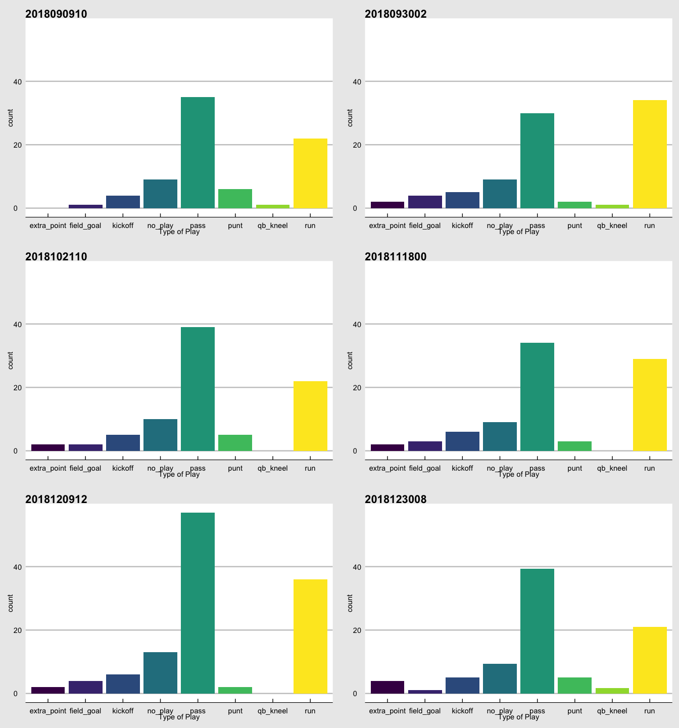
What does Dallas do with the ball?
p <- dal_season %>%  filter(posteam=="DAL") %>% ggplot(aes(x=play_type, fill=play_type)) + geom_bar() + scale_fill_viridis_d(guide=FALSE) + transition_states(game_id) + labs(title = "{closest_state}", x="Type of Play") + theme_economist_white()
animate(p)
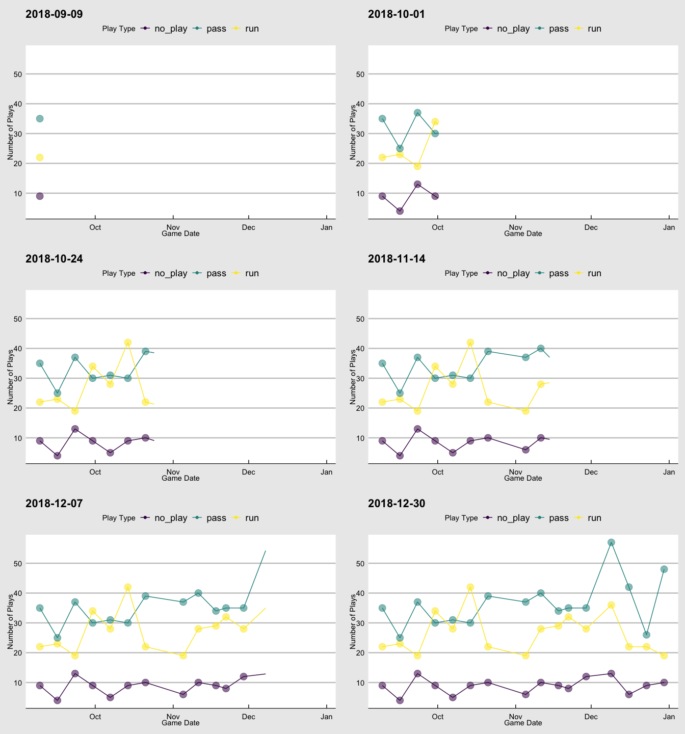
That’s kinda cool. Now I want to clean that up. I do not really want to look at most of the types of possession plays; no play, pass, and run seem interesting, though. Let’s try that out. I also want to change up the display a little bit. Instead of looking at it as a series of graphics, I want the bars to represent the percents from the previous type table and then to show the whole season as it arrives.
dal_RP <- dal_season  %>% filter(posteam=="DAL" & play_type %in% c("no_play","run","pass")) %>% tabyl(game_date, play_type)
dal_RP <-  dal_RP %>% gather("play_type", "count", pass,run,no_play)
p <- dal_RP %>% ggplot(aes(x=game_date, y=count, color=play_type)) + geom_line() + scale_color_viridis_d() +  labs(title = "{frame_along}", y="Number of Plays", color="Play Type", x="Game Date") + theme_economist_white() + geom_point(aes(group=seq_along(game_date), size=1.5, alpha=0.5)) + guides(size=FALSE, alpha=FALSE) + transition_reveal(game_date)
animate(p)
I think that more or less gets what I want. This might also be a cool case for a simple plotly line plot with a hover for the game and details.