Cleaning Messy National Weather Service Data for Portland
Loading NWS Data
I first will try to load it without any intervention to see what it looks like. As we will see, it is quite messy in a few easy ways and a few that are a bit more tricky.
NWS <- read.csv(url("https://www.weather.gov/source/pqr/climate/webdata/Portland_dailyclimatedata.csv"))
head(NWS, 10) %>% kable() %>%
    kable_styling() %>%
scroll_box(width = "100%", height = "500px")| Daily.Temperature.and.Precipitation.Data | X | X.1 | X.2 | X.3 | X.4 | X.5 | X.6 | X.7 | X.8 | X.9 | X.10 | X.11 | X.12 | X.13 | X.14 | X.15 | X.16 | X.17 | X.18 | X.19 | X.20 | X.21 | X.22 | X.23 | X.24 | X.25 | X.26 | X.27 | X.28 | X.29 | X.30 | X.31 | X.32 | X.33 |
|---|---|---|---|---|---|---|---|---|---|---|---|---|---|---|---|---|---|---|---|---|---|---|---|---|---|---|---|---|---|---|---|---|---|---|
| Portland, Oregon Airport | ||||||||||||||||||||||||||||||||||
| Data Starts: | 13 Oct 1940 | END Year: | 2019 | |||||||||||||||||||||||||||||||
| TX is Maximum Temperature (deg F), TX is Minimum Temperature (deg F), PR is Precipitation (inches), SN is Snowfall (inches) | ||||||||||||||||||||||||||||||||||
| Example: High Temperature 23 October 1940 is 58 while low was 53 deg. | ||||||||||||||||||||||||||||||||||
| YR | MO | 1 | 2 | 3 | 4 | 5 | 6 | 7 | 8 | 9 | 10 | 11 | 12 | 13 | 14 | 15 | 16 | 17 | 18 | 19 | 20 | 21 | 22 | 23 | 24 | 25 | 26 | 27 | 28 | 29 | 30 | 31 | AVG or Total | |
| 1940 | 10 | TX | M | M | M | M | M | M | M | M | M | M | M | M | 75 | 70 | 64 | 72 | 72 | 78 | 78 | 64 | 63 | 61 | 58 | 57 | 57 | 57 | 56 | 53 | 59 | 59 | 52 | M |
| 1940 | 10 | TN | M | M | M | M | M | M | M | M | M | M | M | M | 57 | 53 | 52 | 50 | 58 | 58 | 59 | 54 | 48 | 41 | 53 | 48 | 41 | 38 | 37 | 45 | 48 | 50 | 46 | M |
| 1940 | 10 | PR | M | M | M | M | M | M | M | M | M | M | M | M | 0.01 | T | T | 0 | 0.13 | 0 | T | 0.14 | 0.05 | 0 | 0.63 | 1.03 | 0 | 0 | T | 0.18 | 0.58 | 0.5 | 0.25 | M |
| 1940 | 10 | SN | M | M | M | M | M | M | M | M | M | M | M | M | 0 | 0 | 0 | 0 | 0 | 0 | 0 | 0 | 0 | 0 | 0 | 0 | 0 | 0 | 0 | 0 | 0 | 0 | 0 | 0 |
The column names are stored in the seventh row; to properly import this. In addition, there are two missing value codes: M and - that will have to be accounted for. I will use skip to skip the first 6 rows and declare two distinct values to be encoded as missing. Let’s see what we get.
NWS <- read.csv(url("https://www.weather.gov/source/pqr/climate/webdata/Portland_dailyclimatedata.csv"), skip=6, na.strings = c("M","-"))
head(NWS, 10)
## YR MO X X1 X2 X3 X4 X5 X6 X7 X8 X9 X10 X11 X12 X13
## 1 1940 10 TX <NA> <NA> <NA> <NA> <NA> <NA> <NA> <NA> <NA> <NA> <NA> <NA> 75
## 2 1940 10 TN <NA> <NA> <NA> <NA> <NA> <NA> <NA> <NA> <NA> <NA> <NA> <NA> 57
## 3 1940 10 PR <NA> <NA> <NA> <NA> <NA> <NA> <NA> <NA> <NA> <NA> <NA> <NA> 0.01
## 4 1940 10 SN <NA> <NA> <NA> <NA> <NA> <NA> <NA> <NA> <NA> <NA> <NA> <NA> 0
## 5 1940 11 TX 52 53 47 55 51 58 56 50 48 47 46 45 45
## 6 1940 11 TN 40 38 36 32 42 46 46 42 35 34 35 33 34
## 7 1940 11 PR 0.17 0.02 T 0 0.07 0.28 0.85 0.29 0.02 0.01 0.01 0 0
## 8 1940 11 SN 0 0 0 0 0 0 0 0 0 0 0 0 0
## 9 1940 12 TX 51 53 52 51 56 54 50 51 48 50 46 45 43
## 10 1940 12 TN 42 40 42 42 44 37 34 35 32 26 34 28 27
## X14 X15 X16 X17 X18 X19 X20 X21 X22 X23 X24 X25 X26 X27 X28 X29 X30
## 1 70 64 72 72 78 78 64 63 61 58 57 57 57 56 53 59 59
## 2 53 52 50 58 58 59 54 48 41 53 48 41 38 37 45 48 50
## 3 T T 0 0.13 0 T 0.14 0.05 0 0.63 1.03 0 0 T 0.18 0.58 0.5
## 4 0 0 0 0 0 0 0 0 0 0 0 0 0 0 0 0 0
## 5 47 53 49 46 49 46 49 50 44 42 44 51 44 45 59 57 45
## 6 33 28 27 36 30 29 36 33 28 37 35 37 36 38 43 40 39
## 7 0 0 0 0.29 0.01 0 0.37 T 0 0.12 0.62 0 0 0.51 0.89 T T
## 8 0 0 0 0 0 0 0 0 0 0 0 0 0 0 0 0 0
## 9 40 39 39 41 41 45 46 62 60 56 53 54 45 50 51 43 44
## 10 25 29 33 35 34 35 41 39 39 42 42 42 40 38 36 35 37
## X31 AVG.or.Total
## 1 52 <NA>
## 2 46 <NA>
## 3 0.25 <NA>
## 4 0 0
## 5 <NA> 49.1
## 6 <NA> 35.9
## 7 <NA> 4.53
## 8 <NA> 0
## 9 45 48.5
## 10 32 36Two other things are of note. The first one is that R really doesn’t like columns to be named as numbers so we have an X in front of the numeric days. The second is that the column denoting which variable the rows represent is now X. Let me rename X to be Variable.
NWS <- read.csv(url("https://www.weather.gov/source/pqr/climate/webdata/Portland_dailyclimatedata.csv"), skip=6, na.strings = c("M","-")) %>%
  rename(Variable = X)
str(NWS)
## 'data.frame': 3808 obs. of 35 variables:
## $ YR : int 1940 1940 1940 1940 1940 1940 1940 1940 1940 1940 ...
## $ MO : int 10 10 10 10 11 11 11 11 12 12 ...
## $ Variable : chr "TX" "TN" "PR" "SN" ...
## $ X1 : chr NA NA NA NA ...
## $ X2 : chr NA NA NA NA ...
## $ X3 : chr NA NA NA NA ...
## $ X4 : chr NA NA NA NA ...
## $ X5 : chr NA NA NA NA ...
## $ X6 : chr NA NA NA NA ...
## $ X7 : chr NA NA NA NA ...
## $ X8 : chr NA NA NA NA ...
## $ X9 : chr NA NA NA NA ...
## $ X10 : chr NA NA NA NA ...
## $ X11 : chr NA NA NA NA ...
## $ X12 : chr NA NA NA NA ...
## $ X13 : chr "75" "57" "0.01" "0" ...
## $ X14 : chr "70" "53" "T" "0" ...
## $ X15 : chr "64" "52" "T" "0" ...
## $ X16 : chr "72" "50" "0" "0" ...
## $ X17 : chr "72" "58" "0.13" "0" ...
## $ X18 : chr "78" "58" "0" "0" ...
## $ X19 : chr "78" "59" "T" "0" ...
## $ X20 : chr "64" "54" "0.14" "0" ...
## $ X21 : chr "63" "48" "0.05" "0" ...
## $ X22 : chr "61" "41" "0" "0" ...
## $ X23 : chr "58" "53" "0.63" "0" ...
## $ X24 : chr "57" "48" "1.03" "0" ...
## $ X25 : chr "57" "41" "0" "0" ...
## $ X26 : chr "57" "38" "0" "0" ...
## $ X27 : chr "56" "37" "T" "0" ...
## $ X28 : chr "53" "45" "0.18" "0" ...
## $ X29 : chr "59" "48" "0.58" "0" ...
## $ X30 : chr "59" "50" "0.5" "0" ...
## $ X31 : chr "52" "46" "0.25" "0" ...
## $ AVG.or.Total: chr NA NA NA "0" ...It is disappointing that everything is stored as character type. That will prove advantageous in one respect because there is some /A garbage embedded in two of the variables (SN and PR). Here, I will ask R to find all columns that are stored as character and ask it to remove the string.
NWS <- NWS %>% mutate(across(where(is.character), ~str_remove(.x, "/A")))Now, we will have to fix the values T in the precipitation and snow variables [which are currently stored in repeated rows]. Nevertheless, this should give me what I need to create the monthly data.
Monthly Data
Now I will have to facilitate type conversions; the data are currently character instead of numeric. Looking at the data, I think it is reasonable, though not with total certainty, that they should take values bigger than 0 but smaller than the smallest measured values for that Variable; in this case, the smallest values that I note are 0.01. I will (somewhat) arbitrarily set them to 0.005. With that in mind, let’s see if we can create the monthly data by adjusting those values and selecting only the year, the month. the variable, and AVG.or.Total – the last column that contains the average high/low and the total snowfall and precipitation for that month of that year. Finally, let me change the type of that last column to numeric.
# Now to create a Monthly time series.  The first step is to select the four columns
NWS.Monthly.Base <- NWS %>%
  select(YR, MO, Variable, AVG.or.Total) %>%
  mutate(AVG.or.Total = recode(AVG.or.Total, T = "O.005", `T/A` = "O.005")) %>% # Replace the trace amounts with numbers as they are not missing nor are they zero.
  mutate(AVG.or.Total = stringr::str_replace_all(AVG.or.Total, "/A", "")) %>%
  mutate(AVG.or.Total = as.numeric(AVG.or.Total)) # Turn it into numeric
summary(NWS.Monthly.Base)  # Show a summary
## YR MO Variable AVG.or.Total
## Min. :1940 Min. : 1.000 Length:3808 Min. : 0.00
## 1st Qu.:1960 1st Qu.: 3.750 Class :character 1st Qu.: 0.78
## Median :1980 Median : 7.000 Mode :character Median :33.25
## Mean :1980 Mean : 6.508 Mean :28.55
## 3rd Qu.:2000 3rd Qu.:10.000 3rd Qu.:52.50
## Max. :2020 Max. :12.000 Max. :88.10
## NA's :112That seems to work. Two more steps to get a clean monthly dataset. The last step is to create four variables named TX, TN, PR, and SN as unique data.frames. To make merging them by a common index easier, I will use paste to create a character variable of the data and then turn it into a Date: Month.YR.
TX <- NWS.Monthly.Base %>% filter(Variable == "TX") %>%
    mutate(Month.Yr = as.Date(paste0(MO,"-14-",YR), format = "%m-%d-%Y"),
           TX = AVG.or.Total) %>%
    select(-c(Variable,AVG.or.Total))
TN <- NWS.Monthly.Base %>% filter(Variable == "TN") %>%
    mutate(Month.Yr = as.Date(paste0(MO,"-14-",YR), format = "%m-%d-%Y"),
           TN = AVG.or.Total) %>%
    select(-c(Variable,AVG.or.Total))
PR <- NWS.Monthly.Base %>% filter(Variable == "PR") %>%
    mutate(Month.Yr = as.Date(paste0(MO,"-14-",YR), format = "%m-%d-%Y"),
           PR = AVG.or.Total) %>%
    select(-c(Variable,AVG.or.Total))
SN <- NWS.Monthly.Base %>% filter(Variable == "SN") %>%
    mutate(Month.Yr = as.Date(paste0(MO,"-14-",YR), format = "%m-%d-%Y"),
           SN = AVG.or.Total) %>%
    select(-c(Variable,AVG.or.Total))
The last step is to merge the clean individual series together; I will use left_join.
NWS.Monthly.Clean <- left_join(TX,TN) %>% left_join(.,PR) %>% left_join(.,SN)Woo hoo! One down and one to go. But, as we should’ve noticed before, their totals aren’t actually great.
Maximum Temperature
NWS.Monthly.Clean %>% ggplot() + aes(x=Month.Yr, y=TX) + geom_line()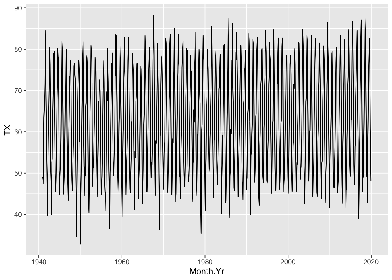
Minimum Temperature
NWS.Monthly.Clean %>% ggplot() + aes(x=Month.Yr, y=TN) + geom_line()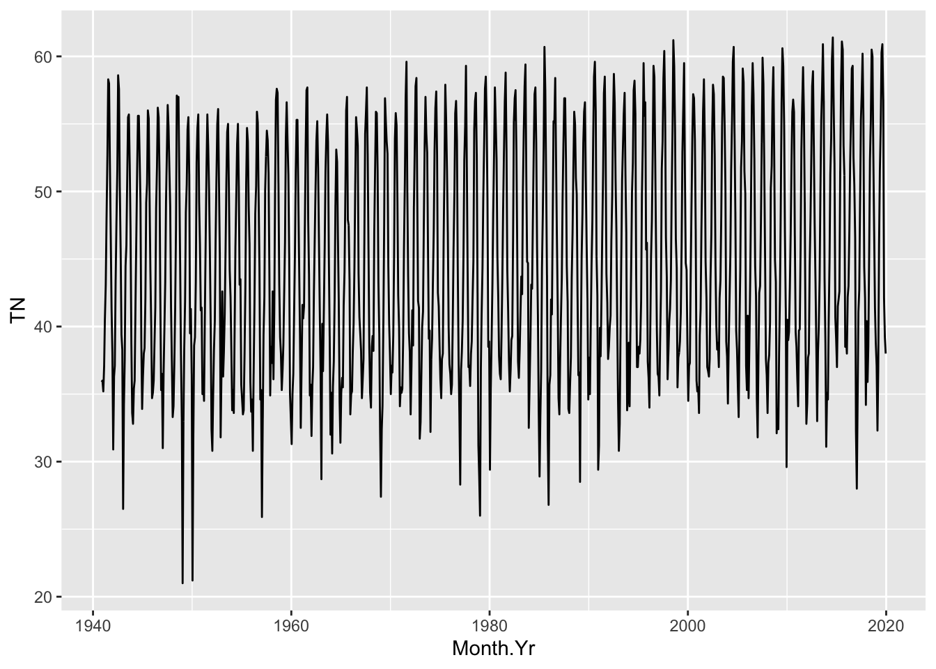
Snow
NWS.Monthly.Clean %>% ggplot() + aes(x=Month.Yr, y=SN) + geom_line()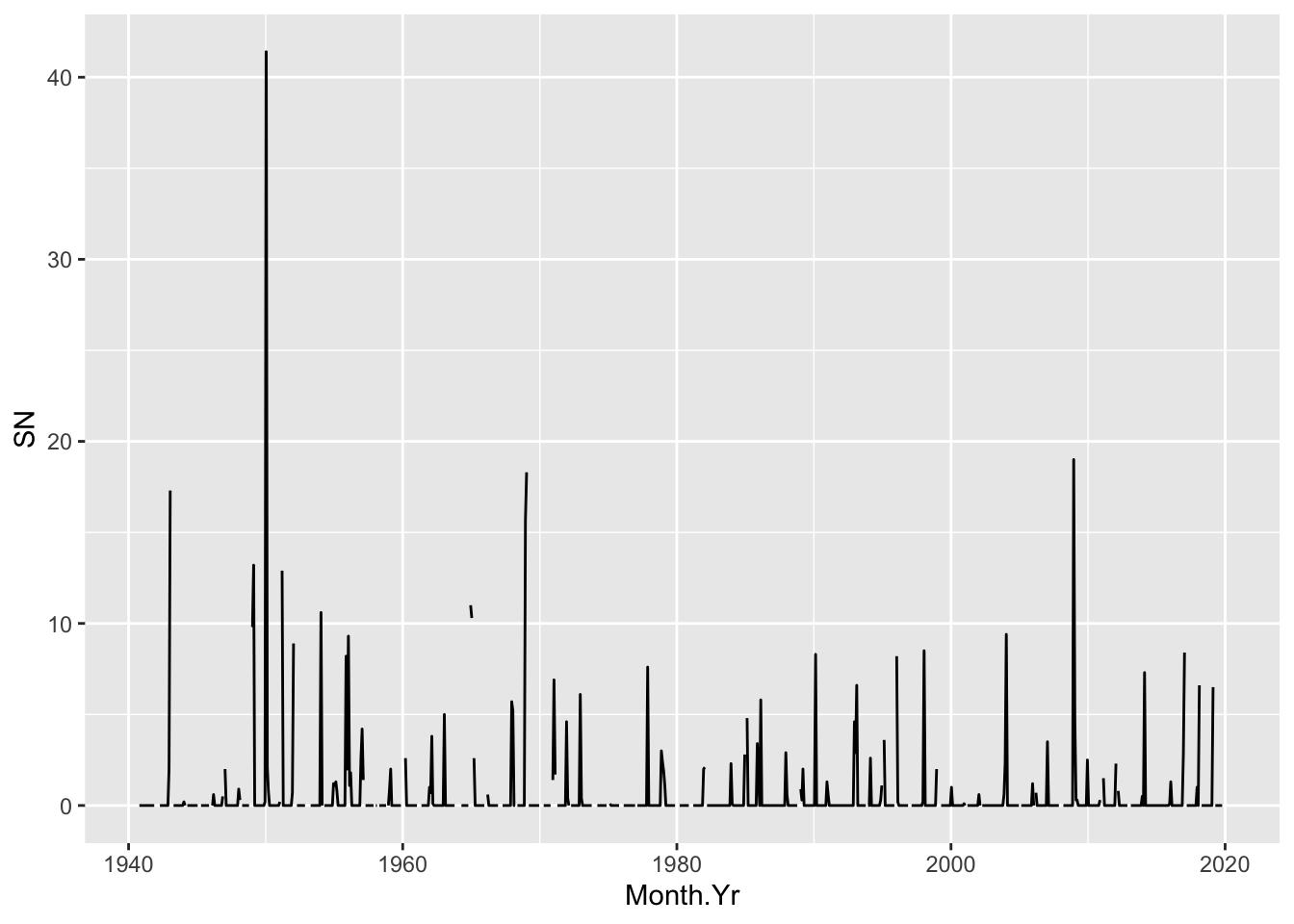
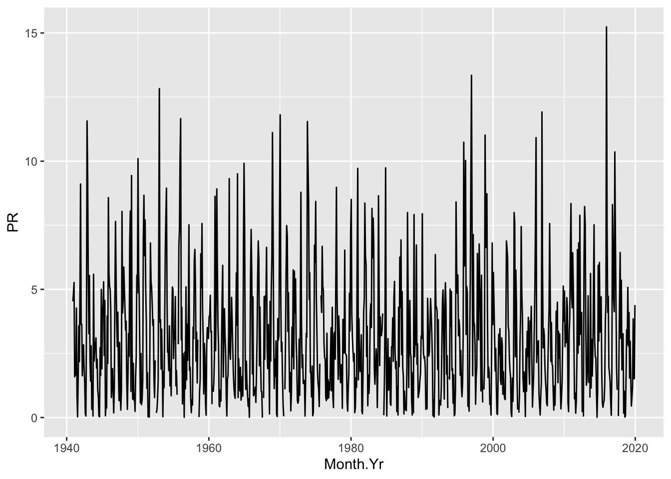
Precipitation
NWS.Monthly.Clean %>% ggplot() + aes(x=Month.Yr, y=PR) + geom_line()