National Weather Service Portland, Part II
Loading NWS Data
I first will try to load it without any intervention to see what it looks like. As we will see, it is quite messy in a few easy ways and a few that are a bit more tricky.
NWS <- read.csv(url("https://www.weather.gov/source/pqr/climate/webdata/Portland_dailyclimatedata.csv"))
head(NWS, 10) %>% kable() %>%
    kable_styling() %>%
scroll_box(width = "100%", height = "500px")| Daily.Temperature.and.Precipitation.Data | X | X.1 | X.2 | X.3 | X.4 | X.5 | X.6 | X.7 | X.8 | X.9 | X.10 | X.11 | X.12 | X.13 | X.14 | X.15 | X.16 | X.17 | X.18 | X.19 | X.20 | X.21 | X.22 | X.23 | X.24 | X.25 | X.26 | X.27 | X.28 | X.29 | X.30 | X.31 | X.32 | X.33 |
|---|---|---|---|---|---|---|---|---|---|---|---|---|---|---|---|---|---|---|---|---|---|---|---|---|---|---|---|---|---|---|---|---|---|---|
| Portland, Oregon Airport | ||||||||||||||||||||||||||||||||||
| Data Starts: | 13 Oct 1940 | END Year: | 2019 | |||||||||||||||||||||||||||||||
| TX is Maximum Temperature (deg F), TX is Minimum Temperature (deg F), PR is Precipitation (inches), SN is Snowfall (inches) | ||||||||||||||||||||||||||||||||||
| Example: High Temperature 23 October 1940 is 58 while low was 53 deg. | ||||||||||||||||||||||||||||||||||
| YR | MO | 1 | 2 | 3 | 4 | 5 | 6 | 7 | 8 | 9 | 10 | 11 | 12 | 13 | 14 | 15 | 16 | 17 | 18 | 19 | 20 | 21 | 22 | 23 | 24 | 25 | 26 | 27 | 28 | 29 | 30 | 31 | AVG or Total | |
| 1940 | 10 | TX | M | M | M | M | M | M | M | M | M | M | M | M | 75 | 70 | 64 | 72 | 72 | 78 | 78 | 64 | 63 | 61 | 58 | 57 | 57 | 57 | 56 | 53 | 59 | 59 | 52 | M |
| 1940 | 10 | TN | M | M | M | M | M | M | M | M | M | M | M | M | 57 | 53 | 52 | 50 | 58 | 58 | 59 | 54 | 48 | 41 | 53 | 48 | 41 | 38 | 37 | 45 | 48 | 50 | 46 | M |
| 1940 | 10 | PR | M | M | M | M | M | M | M | M | M | M | M | M | 0.01 | T | T | 0 | 0.13 | 0 | T | 0.14 | 0.05 | 0 | 0.63 | 1.03 | 0 | 0 | T | 0.18 | 0.58 | 0.5 | 0.25 | M |
| 1940 | 10 | SN | M | M | M | M | M | M | M | M | M | M | M | M | 0 | 0 | 0 | 0 | 0 | 0 | 0 | 0 | 0 | 0 | 0 | 0 | 0 | 0 | 0 | 0 | 0 | 0 | 0 | 0 |
The column names are stored in the seventh row; to properly import this. In addition, there are two missing value codes: M and - that will have to be accounted for. I will use skip to skip the first 6 rows and declare two distinct values to be encoded as missing. Let’s see what we get.
NWS <- read.csv(url("https://www.weather.gov/source/pqr/climate/webdata/Portland_dailyclimatedata.csv"), skip=6, na.strings = c("M","-"))
head(NWS, 10)
## YR MO X X1 X2 X3 X4 X5 X6 X7 X8 X9 X10 X11 X12 X13
## 1 1940 10 TX <NA> <NA> <NA> <NA> <NA> <NA> <NA> <NA> <NA> <NA> <NA> <NA> 75
## 2 1940 10 TN <NA> <NA> <NA> <NA> <NA> <NA> <NA> <NA> <NA> <NA> <NA> <NA> 57
## 3 1940 10 PR <NA> <NA> <NA> <NA> <NA> <NA> <NA> <NA> <NA> <NA> <NA> <NA> 0.01
## 4 1940 10 SN <NA> <NA> <NA> <NA> <NA> <NA> <NA> <NA> <NA> <NA> <NA> <NA> 0
## 5 1940 11 TX 52 53 47 55 51 58 56 50 48 47 46 45 45
## 6 1940 11 TN 40 38 36 32 42 46 46 42 35 34 35 33 34
## 7 1940 11 PR 0.17 0.02 T 0 0.07 0.28 0.85 0.29 0.02 0.01 0.01 0 0
## 8 1940 11 SN 0 0 0 0 0 0 0 0 0 0 0 0 0
## 9 1940 12 TX 51 53 52 51 56 54 50 51 48 50 46 45 43
## 10 1940 12 TN 42 40 42 42 44 37 34 35 32 26 34 28 27
## X14 X15 X16 X17 X18 X19 X20 X21 X22 X23 X24 X25 X26 X27 X28 X29 X30
## 1 70 64 72 72 78 78 64 63 61 58 57 57 57 56 53 59 59
## 2 53 52 50 58 58 59 54 48 41 53 48 41 38 37 45 48 50
## 3 T T 0 0.13 0 T 0.14 0.05 0 0.63 1.03 0 0 T 0.18 0.58 0.5
## 4 0 0 0 0 0 0 0 0 0 0 0 0 0 0 0 0 0
## 5 47 53 49 46 49 46 49 50 44 42 44 51 44 45 59 57 45
## 6 33 28 27 36 30 29 36 33 28 37 35 37 36 38 43 40 39
## 7 0 0 0 0.29 0.01 0 0.37 T 0 0.12 0.62 0 0 0.51 0.89 T T
## 8 0 0 0 0 0 0 0 0 0 0 0 0 0 0 0 0 0
## 9 40 39 39 41 41 45 46 62 60 56 53 54 45 50 51 43 44
## 10 25 29 33 35 34 35 41 39 39 42 42 42 40 38 36 35 37
## X31 AVG.or.Total
## 1 52 <NA>
## 2 46 <NA>
## 3 0.25 <NA>
## 4 0 0
## 5 <NA> 49.1
## 6 <NA> 35.9
## 7 <NA> 4.53
## 8 <NA> 0
## 9 45 48.5
## 10 32 36Two other things are of note. The first one is that R really doesn’t like columns to be named as numbers so we have an X in front of the numeric days. The second is that the column denoting which variable the rows represent is now X. Let me rename X to be Variable.
NWS <- read.csv(url("https://www.weather.gov/source/pqr/climate/webdata/Portland_dailyclimatedata.csv"), skip=6, na.strings = c("M","-")) %>%
  rename(Variable = X)
str(NWS)
## 'data.frame': 3808 obs. of 35 variables:
## $ YR : int 1940 1940 1940 1940 1940 1940 1940 1940 1940 1940 ...
## $ MO : int 10 10 10 10 11 11 11 11 12 12 ...
## $ Variable : chr "TX" "TN" "PR" "SN" ...
## $ X1 : chr NA NA NA NA ...
## $ X2 : chr NA NA NA NA ...
## $ X3 : chr NA NA NA NA ...
## $ X4 : chr NA NA NA NA ...
## $ X5 : chr NA NA NA NA ...
## $ X6 : chr NA NA NA NA ...
## $ X7 : chr NA NA NA NA ...
## $ X8 : chr NA NA NA NA ...
## $ X9 : chr NA NA NA NA ...
## $ X10 : chr NA NA NA NA ...
## $ X11 : chr NA NA NA NA ...
## $ X12 : chr NA NA NA NA ...
## $ X13 : chr "75" "57" "0.01" "0" ...
## $ X14 : chr "70" "53" "T" "0" ...
## $ X15 : chr "64" "52" "T" "0" ...
## $ X16 : chr "72" "50" "0" "0" ...
## $ X17 : chr "72" "58" "0.13" "0" ...
## $ X18 : chr "78" "58" "0" "0" ...
## $ X19 : chr "78" "59" "T" "0" ...
## $ X20 : chr "64" "54" "0.14" "0" ...
## $ X21 : chr "63" "48" "0.05" "0" ...
## $ X22 : chr "61" "41" "0" "0" ...
## $ X23 : chr "58" "53" "0.63" "0" ...
## $ X24 : chr "57" "48" "1.03" "0" ...
## $ X25 : chr "57" "41" "0" "0" ...
## $ X26 : chr "57" "38" "0" "0" ...
## $ X27 : chr "56" "37" "T" "0" ...
## $ X28 : chr "53" "45" "0.18" "0" ...
## $ X29 : chr "59" "48" "0.58" "0" ...
## $ X30 : chr "59" "50" "0.5" "0" ...
## $ X31 : chr "52" "46" "0.25" "0" ...
## $ AVG.or.Total: chr NA NA NA "0" ...It is disappointing that everything is stored as character type. That will prove advantageous in one respect because there is some /A garbage embedded in two of the variables (SN and PR). Here, I will ask R to find all columns that are stored as character and ask it to remove the string.
NWS <- NWS %>% mutate(across(where(is.character), ~str_remove(.x, "/A")))Now, we will have to fix the values T in the precipitation and snow variables [which are currently stored in repeated rows]. Nevertheless, this should give me what I need to create the monthly data.
Daily Data
The daily data will necessarily not involve the column of Totals/Averages that we used for the monthly data so let us eliminate it.
NWS.Daily <- NWS %>% select(-AVG.or.Total)Now I want to rename the columns with names X1, X2, …, X31 to Day.1 to Day.31 for clarity. It is largely inconsequential, it would work on the X’s but I prefer nicely labeled intermediate steps.
names(NWS.Daily) <- c("YR","MO","Variable",paste0("Day.",1:31))The next step is to tidy the data. First, let me use pivot_longer on every column that starts with Day. putting the variable names in Day and variable values in value.
NWS.Daily.Base <- NWS.Daily %>%
  pivot_longer(., cols=starts_with("Day."), names_to = "Day", values_to = "value")
head(NWS.Daily.Base)
## # A tibble: 6 × 5
## YR MO Variable Day value
## <int> <int> <chr> <chr> <chr>
## 1 1940 10 TX Day.1 <NA>
## 2 1940 10 TX Day.2 <NA>
## 3 1940 10 TX Day.3 <NA>
## 4 1940 10 TX Day.4 <NA>
## 5 1940 10 TX Day.5 <NA>
## 6 1940 10 TX Day.6 <NA>Now I want to turn the days into numbers [they are character above] and then use pivot_wider to get the four variables into unique columns, recode trace [T] where they exist to numbers that are half the size of the smallest values, turn them into numbers, and create a date.
NWS.Daily.Base %<>%  mutate(Day = str_remove(Day, "Day.")) %>%
  pivot_wider(., names_from = "Variable", values_from = "value")
NWS.Daily <- NWS.Daily.Base %>% mutate(PR = recode(PR, T = "O.005"), SN = recode(SN, T = "O.005")) %>%
  mutate(TX = as.numeric(TX), TN = as.numeric(TN), PR = as.numeric(PR), SN = as.numeric(SN),
         date = as.Date(paste(MO,Day,YR,sep="-"), format="%m-%d-%Y")
         )
NWS.Daily.Clean <- NWS.Daily %>% filter(!is.na(date))
head(NWS.Daily.Clean)
## # A tibble: 6 × 8
## YR MO Day TX TN PR SN date
## <int> <int> <chr> <dbl> <dbl> <dbl> <dbl> <date>
## 1 1940 10 1 NA NA NA NA 1940-10-01
## 2 1940 10 2 NA NA NA NA 1940-10-02
## 3 1940 10 3 NA NA NA NA 1940-10-03
## 4 1940 10 4 NA NA NA NA 1940-10-04
## 5 1940 10 5 NA NA NA NA 1940-10-05
## 6 1940 10 6 NA NA NA NA 1940-10-06This is exactly what I needed.
Some Plots
By Day?
NWS.Daily.Clean %>% ggplot() + aes(x=date, y=PR) + geom_point(alpha=0.1) + theme_ipsum_rc() + labs(title="Daily Precipitation")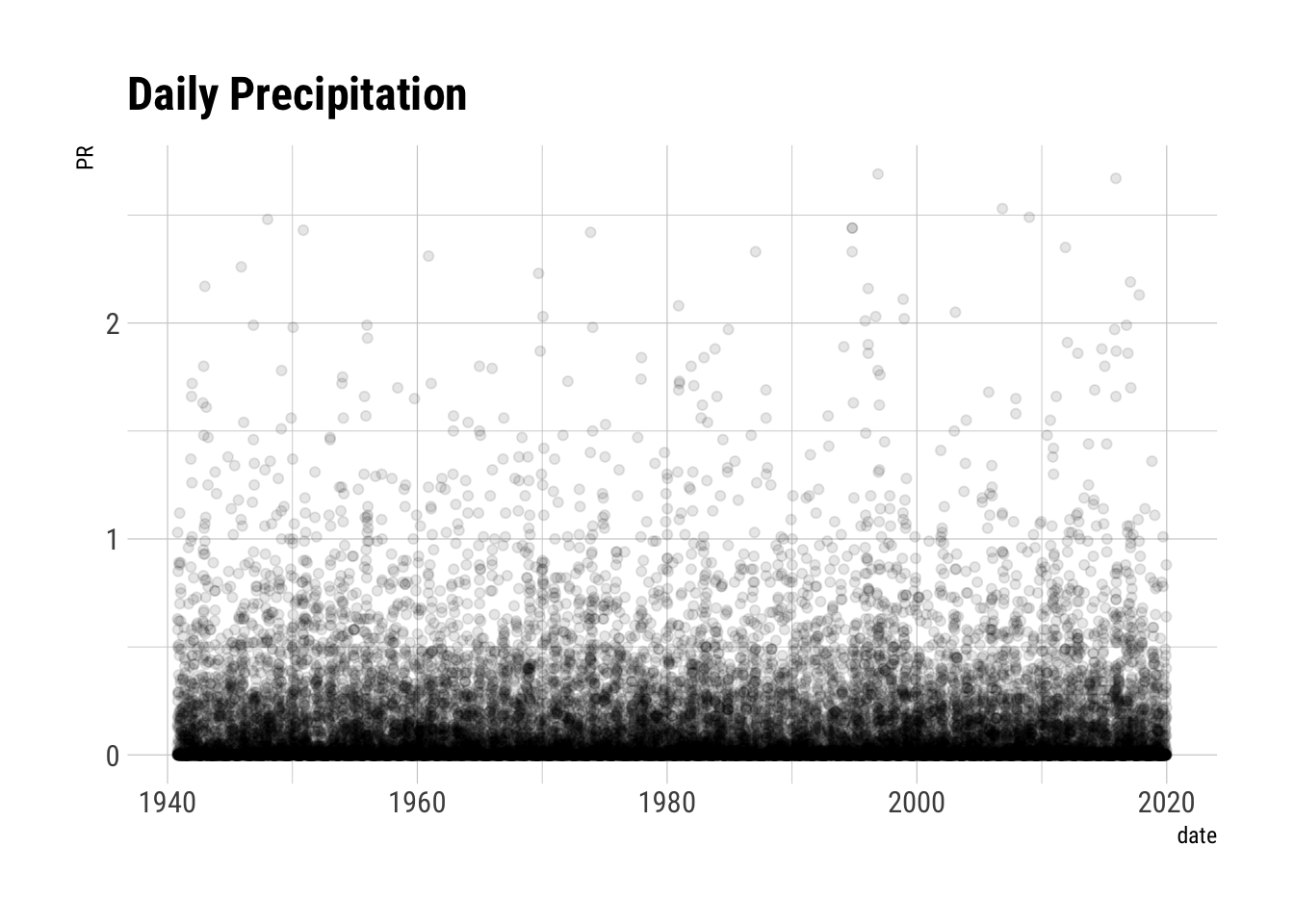
This is really pretty terrible. This is going to need a good bit of work. My first go is going to be to create a moving average that can smooth out the look. I will use a 14-day moving average.
NWS.Daily.Clean %>%
  arrange(date) %>%
  mutate(Rolling.Average = zoo::rollmean(PR, 7, fill=NA)) %>%
  ggplot(., aes(x=date, y=PR)) + geom_point(alpha=0.05, size=0.5) + geom_line(aes(x=date, y=Rolling.Average), inherit.aes=FALSE, color="red") + theme_ipsum_rc() + labs(title="Daily Precipitation")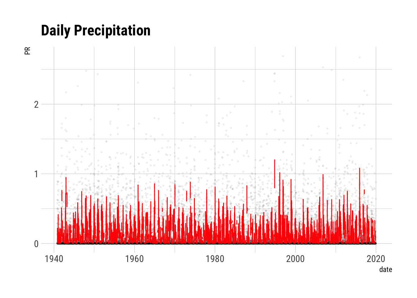
Time Series Plots
Daily
NWS.Daily.Clean <- NWS.Daily.Clean %>% as_tsibble(., index=date)
NWS.Daily.Clean %>% filter(date > "2010-01-01") %>% autoplot(TX) + labs(title="Daily High Temperatures in Portland, Oregon", caption = "Data from NWS", x = "Date", y="High Temperature (deg F)")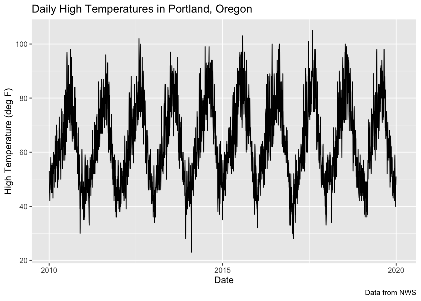
Seasonal Plots
Daily
NWS.Daily.Clean %>% filter(date > "2015-01-01") %>% gg_season(TX, labels = "both")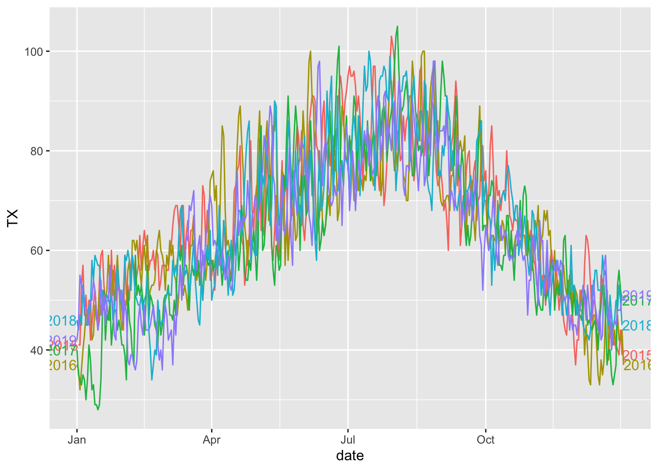
Subseries Plots
Daily
Daily subseries plots are a mess because there are 31 and I am not sure that there would be much instructive anyway as daily variation in temperature is quite noisy.
NWS.Daily.Clean %>% gg_subseries(TX, period="weeks")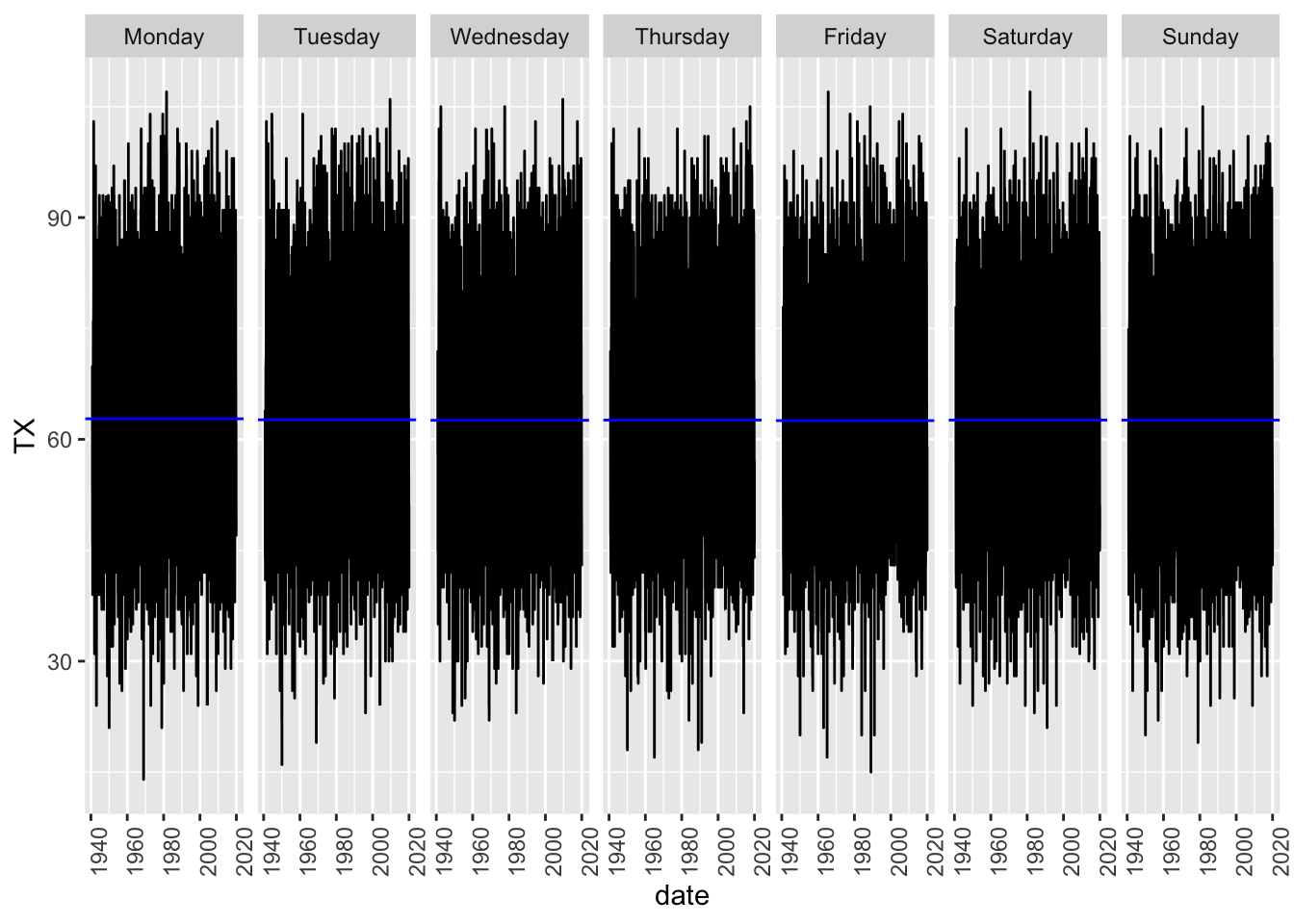
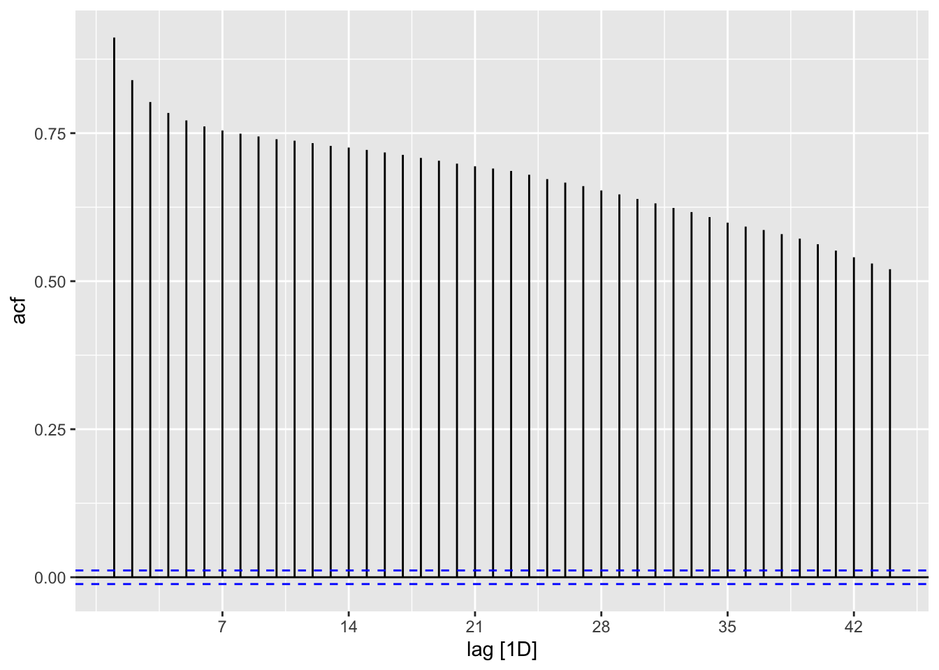
Autocorrelation
To what degree are observations separated by k time periods correlated.
\[r_{k} = \frac{\sum\limits_{t=k+1}^T (y_{t}-\bar{y})(y_{t-k}-\bar{y})} {\sum\limits_{t=1}^T (y_{t}-\bar{y})^2}\] where \(T\) is the length of the time series. The autocorrelation coefficients make up the autocorrelation function or ACF.
The autocorrelation coefficients for the monthly high temperatures can be computed using the ACF() function.
Daily: ACF
NWS.Daily.Clean %>% ACF(TX) %>% autoplot()