Pew Data on Bond Ratings and Rainy Day Funds
Pew on Rainy Day Funds and Credit Quality
The Pew Charitable Trusts released a report last May (2017) that portrays rainy day funds that are well designed and deployed as a form of insurance against ratings downgrades. One the one hand, this is perfectly sensible because the alternatives do not sound like very good ideas. A poorly designed rainy day fund, for example, is going to have to fall short on either the rainy day or the fund. A poorly deployed savings device for cash flow management over the not-so-short term also seems unlikely to bolster market confidence in the repayment abilities of an issuer. If this very simple perspective that seems plausible is true, then a simple replication should be easy. And it is. Pew gladly shared the data and code. If one has access to Stata, the study is easy to replicate.
Taken from the website above:

Pew Recommendations
On the other hand
The variation in the data may leave a good bit to be desired. Let’s have a look at some basic features of the data.
library(haven)
library(dplyr)
library(here)
Pew.Data <- read_dta(url("https://github.com/robertwwalker/academic-mymod/raw/master/data/Pew/modeledforprediction.dta"))
glimpse(Pew.Data)
## Rows: 966
## Columns: 45
## $ fyear <dbl> 1994, 1995, 1996, 1997, 1998, 1999, 2000, 2001, 2002…
## $ statefips <dbl> 1, 1, 1, 1, 1, 1, 1, 1, 1, 1, 1, 1, 1, 1, 1, 1, 1, 1…
## $ state <chr> "Alabama", "Alabama", "Alabama", "Alabama", "Alabama…
## $ bbalance <dbl> 0.00000, 0.00000, 0.00000, 0.00000, 0.00000, 0.00000…
## $ withdraw <dbl> 0.0000, 0.0000, 0.0000, 0.0000, 0.0000, 0.0000, 0.00…
## $ deposit <dbl> 0.000, 0.000, 0.000, 0.000, 0.000, 0.000, 0.000, 0.0…
## $ interest <dbl> 0, 0, 0, 0, 0, 0, 0, 0, 0, 0, 0, 0, 0, 0, 0, 0, 0, 0…
## $ ebalance <dbl> 0.00000, 0.00000, 0.00000, 0.00000, 0.00000, 0.00000…
## $ fund <dbl> 0, 0, 0, 0, 0, 0, 0, 0, 0, 0, 0, 0, 0, 0, 0, 0, 1, 1…
## $ spo <dbl> 0, 0, 0, 0, 0, 0, 0, 0, 0, 0, -1, 0, 0, 0, 0, 0, 0, …
## $ moodyo <dbl> NA, NA, NA, NA, NA, NA, NA, NA, NA, NA, 0, 0, 0, 0, …
## $ fitcho <dbl> NA, NA, NA, NA, NA, NA, NA, NA, NA, NA, NA, NA, 0, 0…
## $ spnum <dbl> 5, 5, 5, 5, 5, 5, 5, 5, 5, 5, 5, 5, 5, 5, 5, 5, 5, 5…
## $ moodynum <dbl> 6, 6, 6, 6, 5, 5, 5, 5, 5, 5, 5, 6, 6, 6, 6, 6, 7, 7…
## $ fitchnum <dbl> 5, 5, 5, 5, 5, 5, 5, 5, 5, 5, 5, 5, 5, 5, 5, 5, 6, 6…
## $ surplus <dbl> -3, -73, 4, -35, 27, 21, 30, -34, -47, -177, 152, 35…
## $ gfebal <dbl> 128, 54, 58, 23, 51, 72, 101, 67, 19, 113, 347, 664,…
## $ longdebt <dbl> 0.10800536, 0.09275389, 0.08864151, 0.08145412, 0.08…
## $ shortdebt <dbl> 2.790155e-05, 8.648518e-05, 7.688679e-06, 4.916201e-…
## $ totaldebt <dbl> 0.10803326, 0.09284038, 0.08864920, 0.08145904, 0.08…
## $ population <dbl> 8.346216, 8.357078, 8.365626, 8.373577, 8.382046, 8.…
## $ pop65 <dbl> 548.045, 554.718, 561.331, 567.094, 571.722, 574.279…
## $ gfe <dbl> 3860, 4151, 4240, 4475, 4688, 4919, 5215, 5213, 5325…
## $ gfr <dbl> 3857, 4078, 4244, 4440, 4715, 4940, 5245, 5179, 5278…
## $ spi <dbl> 79368.02, 84194.33, 88048.51, 92206.95, 98699.30, 10…
## $ rdfbal <dbl> 0.0000000, 0.0000000, 0.0000000, 0.0000000, 0.000000…
## $ rdfdep <dbl> 0.00000, 0.00000, 0.00000, 0.00000, 0.00000, 0.00000…
## $ rdfwit <dbl> 0.000000, 0.000000, 0.000000, 0.000000, 0.000000, 0.…
## $ gfebalgfe <dbl> 3.3160622, 1.3008914, 1.3679246, 0.5139665, 1.087883…
## $ spratingshift <dbl> NA, 0, 0, 0, 0, 0, 0, 0, 0, 0, 0, 0, 0, 0, 0, 0, 0, …
## $ spupgrade <dbl> NA, 0, 0, 0, 0, 0, 0, 0, 0, 0, 0, 0, 0, 0, 0, 0, 0, …
## $ spdowngrade <dbl> NA, 0, 0, 0, 0, 0, 0, 0, 0, 0, 0, 0, 0, 0, 0, 0, 0, …
## $ moodyratingshift <dbl> NA, 0, 0, 0, -1, 0, 0, 0, 0, 0, 0, 1, 0, 0, 0, 0, 1,…
## $ moodyupgrade <dbl> NA, 0, 0, 0, 0, 0, 0, 0, 0, 0, 0, 1, 0, 0, 0, 0, 1, …
## $ moodydowngrade <dbl> NA, 0, 0, 0, 1, 0, 0, 0, 0, 0, 0, 0, 0, 0, 0, 0, 0, …
## $ fitchratingshift <dbl> NA, 0, 0, 0, 0, 0, 0, 0, 0, 0, 0, 0, 0, 0, 0, 0, 1, …
## $ fitchupgrade <dbl> NA, 0, 0, 0, 0, 0, 0, 0, 0, 0, 0, 0, 0, 0, 0, 0, 1, …
## $ fitchdowngrade <dbl> NA, 0, 0, 0, 0, 0, 0, 0, 0, 0, 0, 0, 0, 0, 0, 0, 0, …
## $ rdfnet <dbl> 0.0000, 0.0000, 0.0000, 0.0000, 0.0000, 0.0000, 0.00…
## $ rdfnetgfe <dbl> 0.000000, 0.000000, 0.000000, 0.000000, 0.000000, 0.…
## $ revenuebw <dbl> 4.613832, 15.427544, -32.826214, -55.708824, 5.46266…
## $ revenuebwtrend <dbl> 3852.386, 4062.573, 4276.826, 4495.709, 4709.537, 48…
## $ trendstanding <dbl> 1, 1, -1, -1, 1, 1, 1, 1, -1, -1, -1, -1, 1, 1, 1, -…
## $ valenceusage <dbl> 0.0000, 0.0000, 0.0000, 0.0000, 0.0000, 0.0000, 0.00…
## $ valenceusagegfe <dbl> 0.000000, 0.000000, 0.000000, 0.000000, 0.000000, 0.…table(Pew.Data$state)##
## Alabama Alaska Arizona Arkansas California
## 21 21 21 21 21
## Connecticut Delaware Florida Georgia Hawaii
## 21 21 21 21 21
## Idaho Indiana Iowa Kentucky Louisiana
## 21 21 21 21 21
## Maine Maryland Massachusetts Michigan Minnesota
## 21 21 21 21 21
## Mississippi Missouri Nebraska Nevada New Hampshire
## 21 21 21 21 21
## New Jersey New Mexico New York North Carolina North Dakota
## 21 21 21 21 21
## Ohio Oklahoma Oregon Pennsylvania Rhode Island
## 21 21 21 21 21
## South Carolina South Dakota Tennessee Texas Utah
## 21 21 21 21 21
## Vermont Virginia Washington West Virginia Wisconsin
## 21 21 21 21 21
## Wyoming
## 21The panel is balanced; in the original, New Mexico, New York, South Carolina, and Vermont are duplicated but the Stata code writes out a transformed dataset for analysis that is recorded. The technical report accompanying the study and the stata code give us some insights. In all cases, there are two or more RDF’s and they require combining.
Combining Ratings
In previous work, Skip Krueger and I have treated bond ratings as a multiple rater problem and have deployed cumulative IRT models to measure latent credit quality. One of the methodologically desireable approaches to the Pew study was a model deploying state-level fixed effects but the ordinal data precludes doing this reliably because states that have always experienced the highest rating will have unbounded fixed effects. The continuous latent scale post measurement allows us to sidestep that problem. First, let me scale the data
Scaling the Ratings
library(MCMCpack)
Scaled.BR <- MCMCordfactanal(~spnum+fitchnum+moodynum, data=Pew.Data, factors=1, burnin = 1e6, mcmc=1e6, thin=100, store.scores=TRUE, tune=0.7, lambda.constraints=list(fitchnum=list(2,"+")), verbose=50000)
library(tidyverse)
load(url("https://github.com/robertwwalker/academic-mymod/raw/master/data/Pew/Scaled-BR-Pew.RData"))
state.ratings <- data.frame(state=Pew.Data$state, statefips=Pew.Data$statefips, year=Pew.Data$fyear, BR.Data)
state.ratings.long <- tidyr::gather(state.ratings, sampleno, value, -statefips, -year, -state)
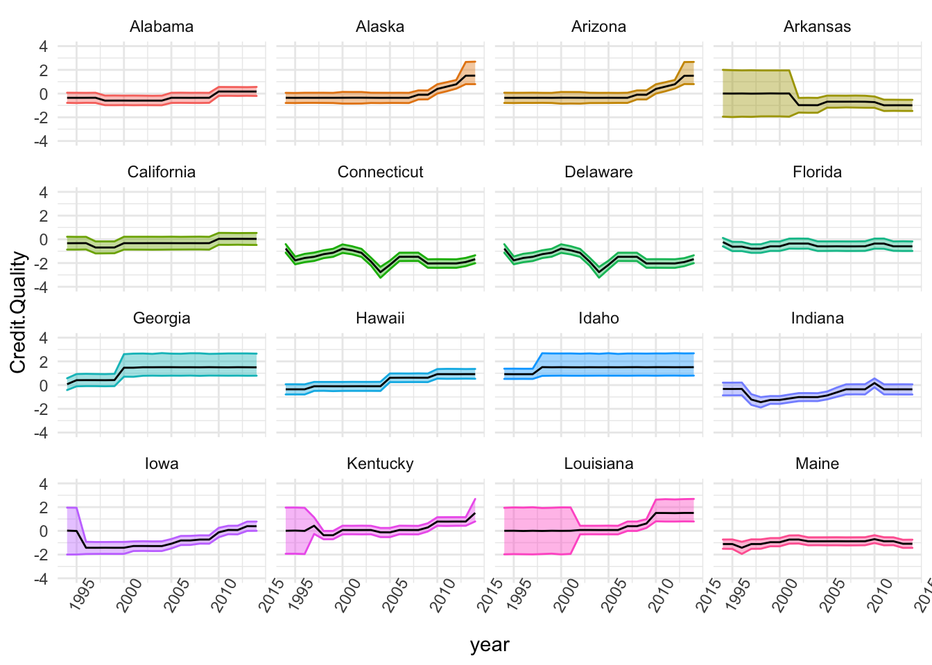
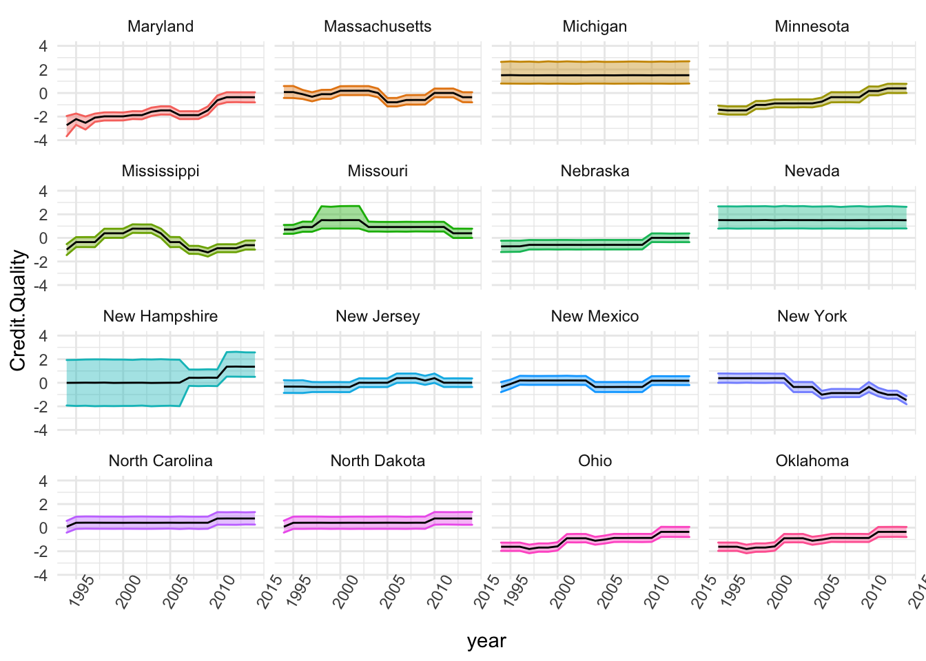
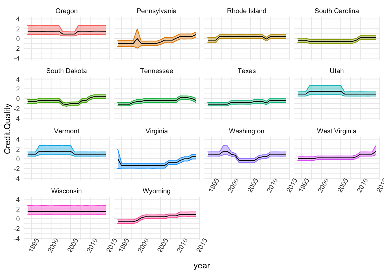
state.SE <- state.ratings.long %>% group_by(state,year) %>% summarise(Credit.Quality=mean(value), t1=quantile(value, probs=0.025), t2=quantile(value, probs=0.975))What does the scaling look like?
The First Group
stored <- list()
stored <- state.SE %>% group_by(state) %>% filter(state%in%c(names(table(state.SE$state))[c(1:16)])) %>%
  ggplot(., aes(x=year, y=Credit.Quality)) + theme_minimal() + theme(axis.text.x  = element_text(angle=60)) +
    geom_ribbon(aes(ymin=t1, ymax=t2, colour=state, fill=state), alpha=0.4) + guides(fill="none", alpha="none") +
    geom_line() + guides(colour="none") +
#    geom_jitter(width=0.2) +
#    geom_point(shape=21, size=3, fill="white") +
    ylim(-4,4) + facet_wrap(~state)
stored
The Second Group
stored <- list()
stored <- state.SE %>% group_by(state) %>% filter(state%in%c(names(table(state.SE$state))[c(17:32)])) %>%
  ggplot(., aes(x=year, y=Credit.Quality)) + theme_minimal() + theme(axis.text.x  = element_text(angle=60)) +
    geom_ribbon(aes(ymin=t1, ymax=t2, colour=state, fill=state), alpha=0.4) + guides(fill="none", alpha="none") +
    geom_line() + guides(colour="none") +
#    geom_jitter(width=0.2) +
#    geom_point(shape=21, size=3, fill="white") +
    ylim(-4,4) + facet_wrap(~state)
stored
The Third Group
stored <- list()
stored <- state.SE %>% group_by(state) %>% filter(state%in%c(names(table(state.SE$state))[c(33:46)])) %>%
  ggplot(., aes(x=year, y=Credit.Quality)) + theme_minimal() + theme(axis.text.x  = element_text(angle=60)) +
    geom_ribbon(aes(ymin=t1, ymax=t2, colour=state, fill=state), alpha=0.4) + guides(fill="none", alpha="none") +
    geom_line() + guides(colour="none") +
#    geom_jitter(width=0.2) +
#    geom_point(shape=21, size=3, fill="white") +
    ylim(-4,4) + facet_wrap(~state)
stored
The Panel Data Properties
Panel data estmators for linear problems benefit from a very useful decomposition from ANOVA. The total variation in a variable can be decomposed into two components: a within-unit or short-run component and a between-unit averages component (that is constant for any given unit). It is always important, as emphasised in the modelling in Mundlak (1977), to consider the variance components because they conttribute insights into the nature of inferences by telling us how much information and of what sort is contained in each indicator. The number of controls in the study is manageable so in depth analysis is possible.
Analysing the Scaled Data
With continuous measures on the response imputed over 10,000 samples, we can turn to an analysis of these samples to reexamine the dynamics of rainy day fund expenditures on bond ratings.
library(haven)
nlswork <- read_stata("http://www.stata-press.com/data/r13/nlswork.dta")
library(dplyr)
XTSUM <- function(data, varname, unit) {
  varname <- enquo(varname)
  unit <- enquo(unit)
  ores <- nlswork %>% summarise(ovr.mean=mean(!! varname, na.rm=TRUE), ovr.sd=sd(!! varname, na.rm=TRUE), ovr.min = min(!! varname, na.rm=TRUE), ovr.max=max(!! varname, na.rm=TRUE), N.overall=sum(as.numeric(!is.na(!! varname))))
  bmeans <- nlswork %>% group_by(!!unit) %>% summarise(meanx=mean(!! varname, na.rm=T), t.count=sum(as.numeric(!is.na(!! varname))))
  bres <- bmeans %>% summarise(between.sd = sd(meanx, na.rm=TRUE), between.min = min(meanx, na.rm=TRUE), between.max=max(meanx, na.rm=TRUE), t.bar=mean(t.count, na.rm=TRUE), Groups=n())
  wdat <- nlswork %>% group_by(!!unit) %>% mutate(W.x = scale(!! varname, scale=FALSE))
  wres <- wdat %>% ungroup() %>% summarise(within.sd=sd(W.x, na.rm=TRUE), within.min=min(W.x, na.rm=TRUE), within.max=max(W.x, na.rm=TRUE))
  return(list(ores=ores,bres=bres,wres=wres))
}
XTSUM(nlswork, varname=hours, unit=idcode)
## $ores
## # A tibble: 1 x 5
## ovr.mean ovr.sd ovr.min ovr.max N.overall
## <dbl> <dbl> <dbl> <dbl> <dbl>
## 1 36.6 9.87 1 168 28467
##
## $bres
## # A tibble: 1 x 5
## between.sd between.min between.max t.bar Groups
## <dbl> <dbl> <dbl> <dbl> <int>
## 1 7.85 1 83.5 6.04 4711
##
## $wres
## # A tibble: 1 x 3
## within.sd within.min within.max
## <dbl> <dbl> <dbl>
## 1 7.52 -38.7 93.5