Oregon County Support for Retaining Slavery in the OR Constitution
Last update: November 15. 2022
In preparation for the dumpster fire that is Oregon election reporting, I previously posed on importing a directory of .csv files. At present, that is what I can find to build this. What does the interface look like?
library(magick)
Img <- image_read("./img/SShot.png")
image_ggplot(Img)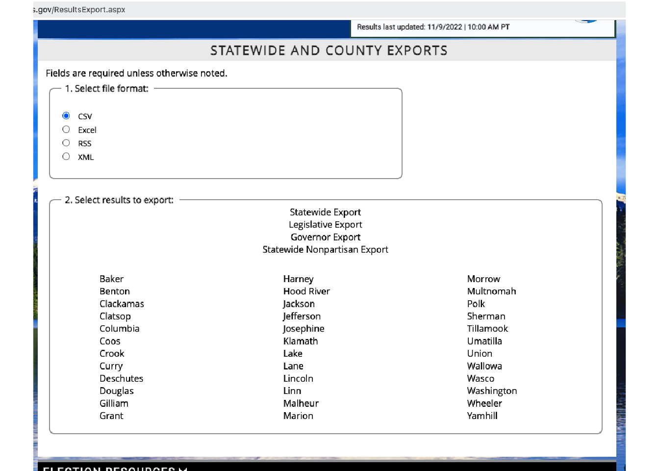
This is terrible, there is a javascript button to download each separately. Nevertheless, here we go.
First, to import the various files. I am going to use an import then export trick to make this easier. First, let me use the directory to create the county names.
library(magrittr); library(tidyverse); library(ggthemes)
filenames <- dir("./data/") %>% data.frame(File.Names = .)
filenames %<>% mutate(County.Names = str_remove(File.Names, ".csv"))
filenames$County.Names
## [1] "Baker" "Benton" "Clackamas" "Clatsop" "Columbia"
## [6] "Coos" "Crook" "Curry" "Deschutes" "Douglas"
## [11] "Gilliam" "Grant" "Harney" "Hood River" "Jackson"
## [16] "Jefferson" "Josephine" "Klamath" "Lake" "Lane"
## [21] "Lincoln" "Linn" "Malheur" "Marion" "Morrow"
## [26] "Multnomah" "Polk" "Sherman" "Tillamook" "Umatilla"
## [31] "Union" "Wallowa" "Wasco" "Washington" "Wheeler"
## [36] "Yamhill"With that I can pull in each file, add the county name to it, and save it back.
c(1:36) %>% walk(., ~ {read_csv(paste0("./data/",filenames$File.Names[.x], sep="")) %>% mutate(County = filenames$County.Names[.x]) %>% write.csv(., file=paste0("./data/",filenames$File.Names[.x], sep=""), row.names=FALSE)})Now to use these to create the data.
Oregon.County.Results <- c(1:36) %>% map_dfr(., ~ read_csv(paste0("./data/",filenames$File.Names[.x], sep="")))What does it look like?
head(Oregon.County.Results)## # A tibble: 6 × 16
## ContestID ContestName Nomin…¹ Party…² AreaT…³ AreaNum Offic…⁴ Ballo…⁵ Candi…⁶
## <dbl> <chr> <chr> <lgl> <lgl> <chr> <dbl> <lgl> <dbl>
## 1 100051746 US Senator <NA> NA NA Federal 1 NA 9.90e3
## 2 100051746 US Senator Democr… NA NA Federal 1 NA 3.00e8
## 3 100051746 US Senator Pacifi… NA NA Federal 1 NA 1.00e8
## 4 100051746 US Senator Progre… NA NA Federal 1 NA 1.00e8
## 5 100051746 US Senator Republ… NA NA Federal 1 NA 1.00e8
## 6 100051748 US Represen… <NA> NA NA US Rep… 2 NA 9.90e3
## # … with 7 more variables: CandidateName <chr>, CurrentDateTime <chr>,
## # VoteFor <dbl>, CandidateVotes <dbl>, CandidatePercentage <dbl>,
## # PrecinctsReporting <chr>, County <chr>, and abbreviated variable names
## # ¹NominatingParty, ²PartyCode, ³AreaType, ⁴OfficeSeqNo, ⁵BallotOrder,
## # ⁶CandidateIDPeeling the results of interest
Slavery.Res <- Oregon.County.Results %>%
  filter(ContestID==100002574 & CandidateName=="No") %>%
  select(County, CandidatePercentage)
library(tigris); library(rgdal); library(htmltools); library(viridis); library(sf); library(ggrepel)
counties.t <- counties(state = "41", resolution = "500k", class="sf")
Map.Me <- left_join(counties.t,Slavery.Res, by=c("NAME" = "County"))
Now to map it.
My.Map <- Map.Me %>%
  ggplot(., aes(geometry=geometry, fill=CandidatePercentage, label=NAME, group=NAME)) +
  geom_sf() +
  geom_label_repel(stat = "sf_coordinates",
    min.segment.length = 0,
    colour = "white",
    segment.colour = "white",
    size = 1,
    box.padding = unit(0.05, "lines")) +
  scale_fill_continuous_tableau("Red") +
  theme_minimal() +
  labs(title="Remove Slavery Measure from Oregon Constitution",
       x="",
       y="",
       fill="Percentage No's")
Here is the map.
My.Map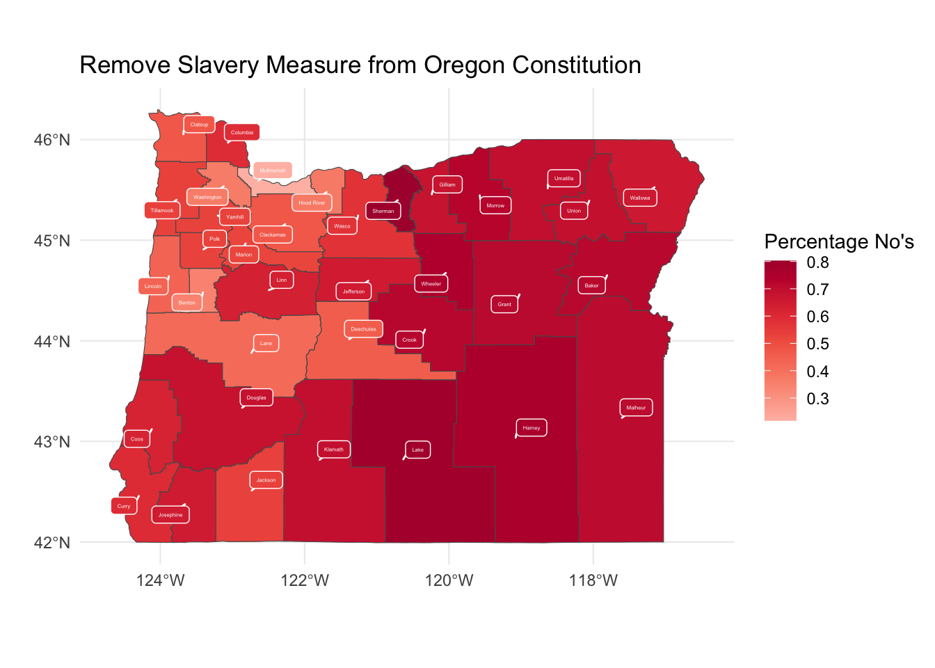
A Regression
I want to estimate a simple regression on some of these data; how much of the variance in No votes for removing slavery from the Oregon Constitution can be explained by support for Christine Drazan.
Oregon.County.Results %>%
  filter((ContestID==100002574 & CandidateName=="No") | CandidateName=="Christine Drazan") %>%
  select(County, CandidatePercentage, CandidateName) %>%
  pivot_wider(., names_from="CandidateName", values_from="CandidatePercentage") %>%
  lm(`No` ~ `Christine Drazan`, data=.) %>% summary
##
## Call:
## lm(formula = No ~ `Christine Drazan`, data = .)
##
## Residuals:
## Min 1Q Median 3Q Max
## -0.037100 -0.020341 -0.005199 0.011769 0.074723
##
## Coefficients:
## Estimate Std. Error t value Pr(>|t|)
## (Intercept) 0.08045 0.01956 4.114 0.000233 ***
## `Christine Drazan` 0.88101 0.03261 27.020 < 2e-16 ***
## ---
## Signif. codes: 0 '***' 0.001 '**' 0.01 '*' 0.05 '.' 0.1 ' ' 1
##
## Residual standard error: 0.03019 on 34 degrees of freedom
## Multiple R-squared: 0.9555, Adjusted R-squared: 0.9542
## F-statistic: 730.1 on 1 and 34 DF, p-value: < 2.2e-16Whoa! Almost 96% using the current totals as of 10AM on the day after the election.
library(emoGG)
Oregon.County.Results %>%
  filter((ContestID==100002574 & CandidateName=="No") | CandidateName=="Christine Drazan") %>%
  select(County, CandidatePercentage, CandidateName) %>%
  pivot_wider(., names_from="CandidateName", values_from="CandidatePercentage") %>%
  ggplot() +
  aes(x=`Christine Drazan`, y=No) +
  geom_point(color="purple") +
  geom_smooth(method="lm") +
  theme_minimal() +
  labs(y="No to Removing Slavery")
## `geom_smooth()` using formula = 'y ~ x'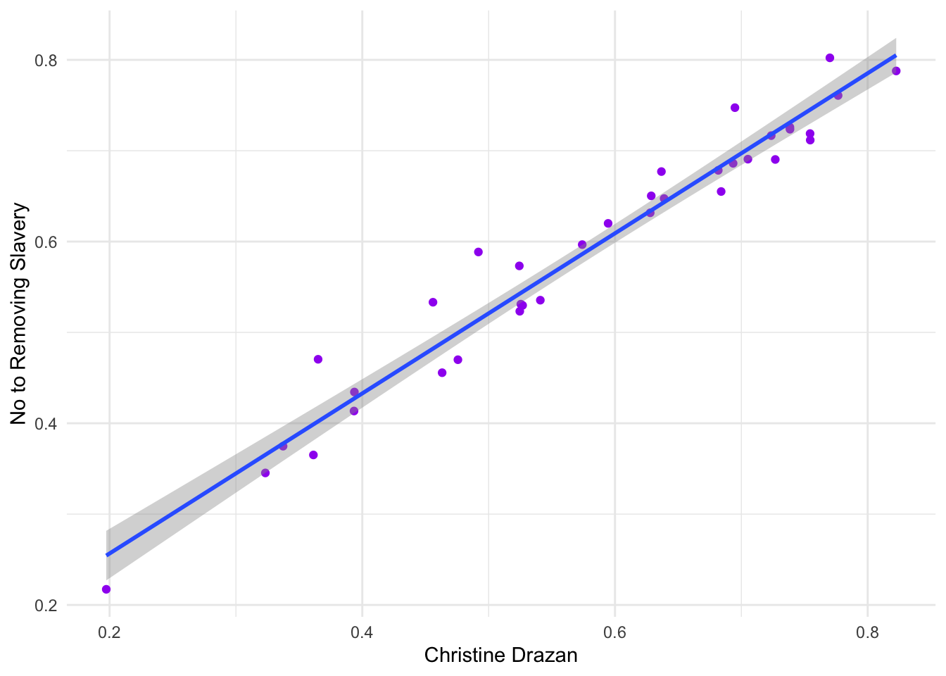
library(plotly)
Oregon.County.Results %>%
  filter((ContestID==100002574 & CandidateName=="No") | CandidateName=="Christine Drazan") %>%
  select(County, CandidatePercentage, CandidateName) %>%
  pivot_wider(., names_from="CandidateName", values_from="CandidatePercentage") %>%
  ggplot() +
  aes(x=`Christine Drazan`, y=No, label=County) +
  geom_point() +
  geom_smooth(method="lm") + theme_minimal() +
  labs(y="Proportion No Votes on Slavery Removal", x="Drazan Vote Proportion", title="Removing Slavery for Convicts from Oregon's Constitution and Drazan Vote", subtitle="By Oregon County, Correlation: 0.9775") -> pgg
pgg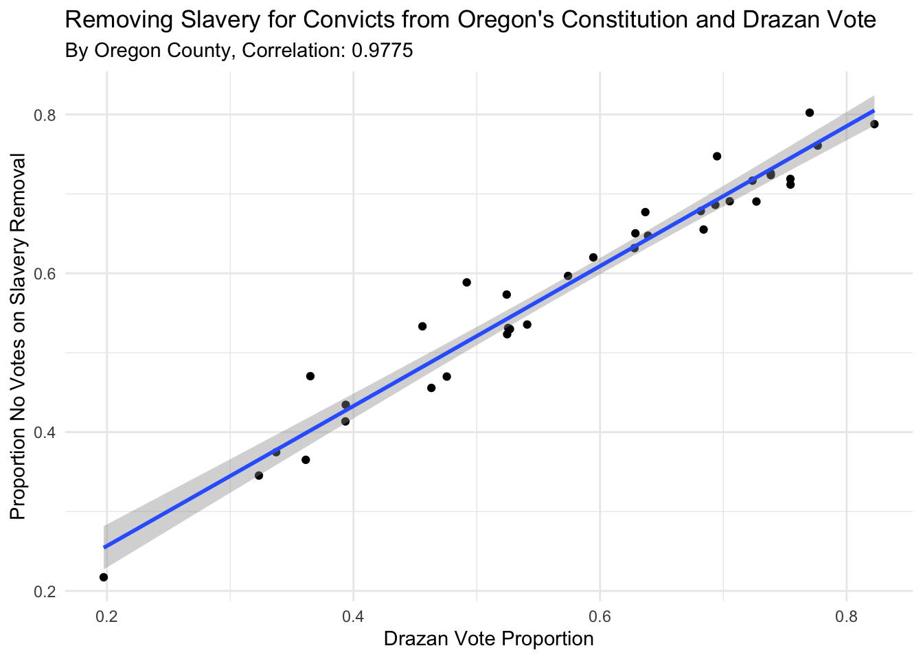
As a plotly
ggplotly(pgg)## `geom_smooth()` using formula = 'y ~ x'## Warning: The following aesthetics were dropped during statistical transformation: label
## ℹ This can happen when ggplot fails to infer the correct grouping structure in
## the data.
## ℹ Did you forget to specify a `group` aesthetic or to convert a numerical
## variable into a factor?