tT: Spending on Kids
Spending on Kids
The Urban Institute has a collection of data on government spending on children. The tidyTuesday page links to some of their commentary and to an article from Governing on the subject. The data are rich and interesting and are conveniently packaged into the tidykids package for R. My goal is to combine geofacets with animation to produce an animation of education spending over time by US states and territories.
First, let me import the data.
kids <- read.csv('https://raw.githubusercontent.com/rfordatascience/tidytuesday/master/data/2020/2020-09-15/kids.csv')
# kids <- readr::read_csv('https://raw.githubusercontent.com/rfordatascience/tidytuesday/master/data/2020/2020-09-15/kids.csv')
Now let me summarise it and show a table of the variables.
summary(kids)## state variable year raw
## Length:23460 Length:23460 Min. :1997 Min. : -60139
## Class :character Class :character 1st Qu.:2002 1st Qu.: 71985
## Mode :character Mode :character Median :2006 Median : 252002
## Mean :2006 Mean : 1181359
## 3rd Qu.:2011 3rd Qu.: 836324
## Max. :2016 Max. :83666088
## NA's :102
## inf_adj inf_adj_perchild
## Min. : -60799 Min. :-0.01361
## 1st Qu.: 85876 1st Qu.: 0.12456
## Median : 298778 Median : 0.32757
## Mean : 1359983 Mean : 0.91448
## 3rd Qu.: 985049 3rd Qu.: 0.83362
## Max. :84584960 Max. :20.27326
## NA's :102 NA's :102A table of the variables. The definitions are best found here.
table(kids$variable)##
## addCC CTC edservs edsubs fedEITC
## 1020 1020 1020 1020 1020
## fedSSI HCD HeadStartPriv highered lib
## 1020 1020 1020 1020 1020
## Medicaid_CHIP other_health othercashserv parkrec pell
## 1020 1020 1020 1020 1020
## PK12ed pubhealth SNAP socsec stateEITC
## 1020 1020 1020 1020 1020
## TANFbasic unemp wcomp
## 1020 1020 1020It is very tidy. It is probably better shown after a pivot. 50 states, the District of Columbia, and 20 years gives us 1,020 observations. Let me show it wide.
Big.Wide <- pivot_wider(kids, id_cols = c(state,year), names_from = "variable", values_from = c("raw","inf_adj","inf_adj_perchild"))
Big.Wide
## # A tibble: 1,020 x 71
## state year raw_PK12ed raw_highered raw_edsubs raw_edservs raw_pell
## <chr> <int> <dbl> <dbl> <dbl> <dbl> <dbl>
## 1 Alab… 1997 3271969 956505 107733 246057 120833.
## 2 Alas… 1997 1042311 209433 5550 52355 7575.
## 3 Ariz… 1997 3388165 847032 111735 170281 120450.
## 4 Arka… 1997 1960613 457171 62447 189808 65904.
## 5 Cali… 1997 28708364 6858657 1121672 943805 775292.
## 6 Colo… 1997 3332994 861733 84129 77419 79004.
## 7 Conn… 1997 4014870 502177 71053 138932 36453.
## 8 Dela… 1997 776825 185114 31284 81880 9965.
## 9 Dist… 1997 544051 56693 0 0 18972.
## 10 Flor… 1997 11498394 2039186 391935 269777 318611.
## # … with 1,010 more rows, and 64 more variables: raw_HeadStartPriv <dbl>,
## # raw_TANFbasic <dbl>, raw_othercashserv <dbl>, raw_SNAP <dbl>,
## # raw_socsec <dbl>, raw_fedSSI <dbl>, raw_fedEITC <dbl>, raw_CTC <dbl>,
## # raw_addCC <dbl>, raw_stateEITC <dbl>, raw_unemp <dbl>, raw_wcomp <dbl>,
## # raw_Medicaid_CHIP <dbl>, raw_pubhealth <dbl>, raw_other_health <dbl>,
## # raw_HCD <dbl>, raw_lib <dbl>, raw_parkrec <dbl>, inf_adj_PK12ed <dbl>,
## # inf_adj_highered <dbl>, inf_adj_edsubs <dbl>, inf_adj_edservs <dbl>,
## # inf_adj_pell <dbl>, inf_adj_HeadStartPriv <dbl>, inf_adj_TANFbasic <dbl>,
## # inf_adj_othercashserv <dbl>, inf_adj_SNAP <dbl>, inf_adj_socsec <dbl>,
## # inf_adj_fedSSI <dbl>, inf_adj_fedEITC <dbl>, inf_adj_CTC <dbl>,
## # inf_adj_addCC <dbl>, inf_adj_stateEITC <dbl>, inf_adj_unemp <dbl>,
## # inf_adj_wcomp <dbl>, inf_adj_Medicaid_CHIP <dbl>, inf_adj_pubhealth <dbl>,
## # inf_adj_other_health <dbl>, inf_adj_HCD <dbl>, inf_adj_lib <dbl>,
## # inf_adj_parkrec <dbl>, inf_adj_perchild_PK12ed <dbl>,
## # inf_adj_perchild_highered <dbl>, inf_adj_perchild_edsubs <dbl>,
## # inf_adj_perchild_edservs <dbl>, inf_adj_perchild_pell <dbl>,
## # inf_adj_perchild_HeadStartPriv <dbl>, inf_adj_perchild_TANFbasic <dbl>,
## # inf_adj_perchild_othercashserv <dbl>, inf_adj_perchild_SNAP <dbl>,
## # inf_adj_perchild_socsec <dbl>, inf_adj_perchild_fedSSI <dbl>,
## # inf_adj_perchild_fedEITC <dbl>, inf_adj_perchild_CTC <dbl>,
## # inf_adj_perchild_addCC <dbl>, inf_adj_perchild_stateEITC <dbl>,
## # inf_adj_perchild_unemp <dbl>, inf_adj_perchild_wcomp <dbl>,
## # inf_adj_perchild_Medicaid_CHIP <dbl>, inf_adj_perchild_pubhealth <dbl>,
## # inf_adj_perchild_other_health <dbl>, inf_adj_perchild_HCD <dbl>,
## # inf_adj_perchild_lib <dbl>, inf_adj_perchild_parkrec <dbl>My brief plan
I recently came across a geofacet for R. I want to use it to plot a little bit of this data. If you want to get a head start, try install.packages("geofacet", dependencies=TRUE). You can google geofacet to get an idea of what a geofacet plot is. I will build one on the fly using a couple of tidy tools: filter, mutate, and joins and then put it together.
library(viridis)## Loading required package: viridisLitelibrary(geofacet)
state_ranks %>% filter(variable=="education") %>% select(state,name) -> mergeMe
p1 <- kids %>%
left_join(., mergeMe, by = c('state' = 'name')) %>%
filter(variable=="PK12ed")%>%
ggplot(., aes(x=year, y=inf_adj_perchild, color=inf_adj_perchild)) +
geom_line() +
facet_geo(~state.y) +
labs(x="year", y="Inflation Adjust Expenditures per child", title="Pre-K Through 12 Education Spending", color="Spend per child", caption="Data from #tidyTuesday: @PieRatio") +
scale_color_viridis_c() + theme_void()
p1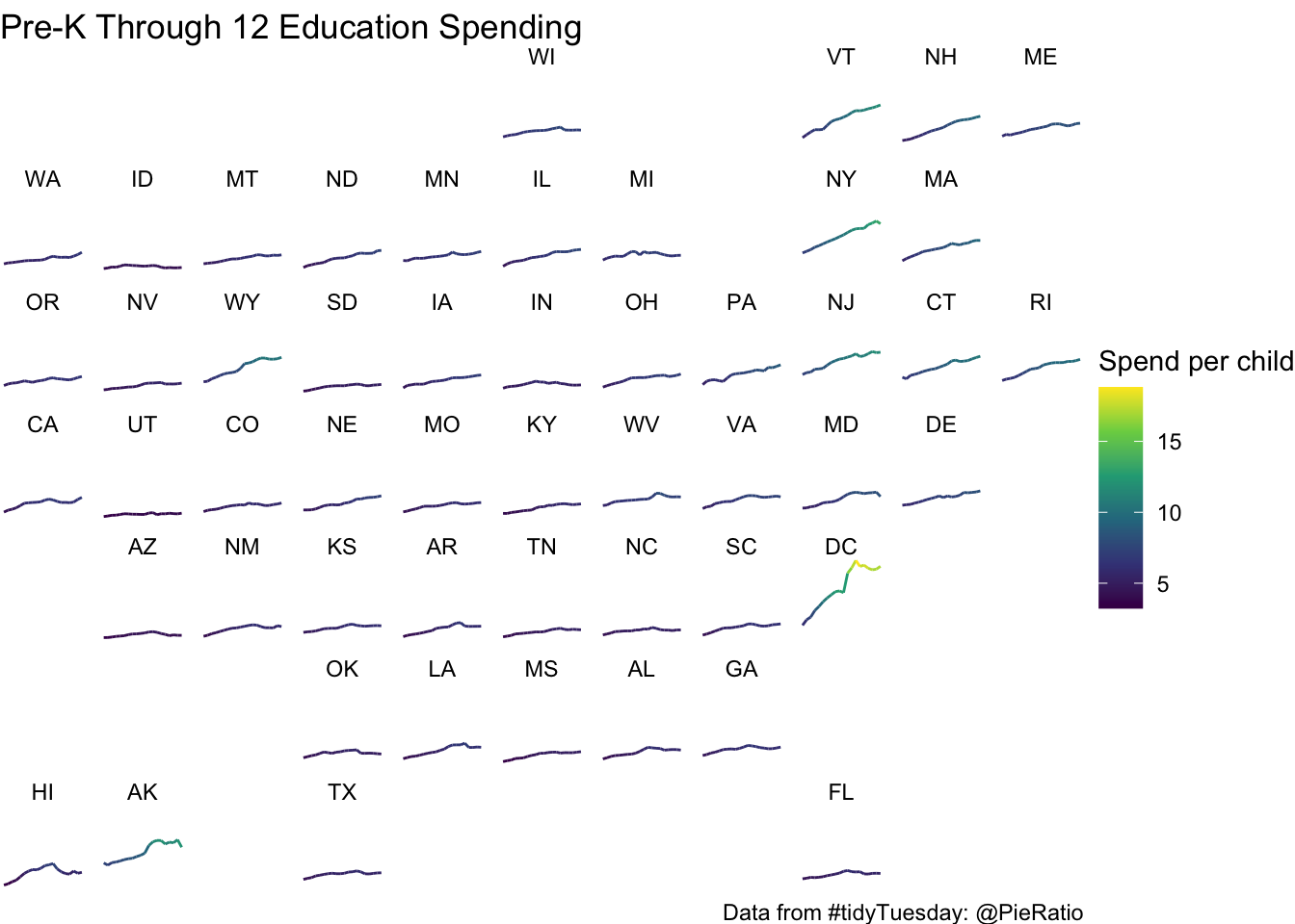
An Animation
library(gganimate)
p2 <- p1 + transition_reveal(year)
p3 <- animate(p2, renderer = gifski_renderer())
save_animation(p3, file = "./GeoAnimFacet.gif")
Animation
Neat-o an Oregon Grid
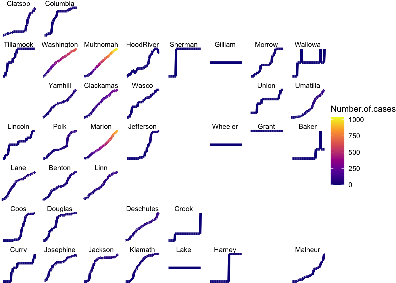
This isn’t very good though…. A basic visualization using geofacet on Oregon COVID data.
load(url("https://github.com/robertwwalker/rww-science/raw/master/content/R/COVID/data/OregonCOVID2020-09-15.RData"))
OR.County.COVID %>%
  mutate(County = str_replace(County, " ", "")) %>%
  ggplot(., aes(x=date, y=Number.of.cases, color=Number.of.cases)) +
  geom_line(size=1.5) +
  facet_geo(~ County, grid = "us_or_counties_grid1", label = "name", scales = "free_y") +
  scale_color_viridis_c(option = "plasma") +
  theme_void()
## Warning: Removed 3 row(s) containing missing values (geom_path).