Stocks and gganimate
tidyquant
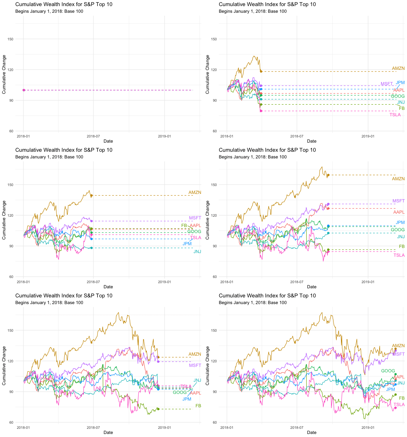
Automates a lot of equity research and calculation using tidy concepts. Here, I will first use it to get the components of the S and P 500 and pick out those with weights over 1.25 percent. In the next step, I download the data and finally calculate daily returns and a cumulative wealth index.
library(tidyquant)
library(tidyverse)
tq_index("SP500") %>% filter(weight > 0.0125) %>% select(symbol,company) -> Tickers
Tickers <- Tickers %>% filter(symbol!="BRK.B") %>% filter(symbol!="GOOGL")
Eq.P <- Tickers %>%  tq_get(., from="2018/01/01", to="2019/03/14")
Returns <- Eq.P %>% group_by(symbol) %>% tq_transmute(., adjusted, periodReturn, period="daily")
C.Returns <- Eq.P %>%
  group_by(symbol) %>%
  tq_transmute(., adjusted, periodReturn, period="daily", type = "log", col_rename = "returns") %>%
  mutate(wealth.index = 100 * cumprod(1 + returns))
library(skimr)
Returns %>% skim()| Name | Piped data |
| Number of rows | 2400 |
| Number of columns | 3 |
| _______________________ | |
| Column type frequency: | |
| Date | 1 |
| numeric | 1 |
| ________________________ | |
| Group variables | symbol |
Variable type: Date
| skim_variable | symbol | n_missing | complete_rate | min | max | median | n_unique |
|---|---|---|---|---|---|---|---|
| date | AAPL | 0 | 1 | 2018-01-02 | 2019-03-13 | 2018-08-06 | 300 |
| date | AMZN | 0 | 1 | 2018-01-02 | 2019-03-13 | 2018-08-06 | 300 |
| date | FB | 0 | 1 | 2018-01-02 | 2019-03-13 | 2018-08-06 | 300 |
| date | GOOG | 0 | 1 | 2018-01-02 | 2019-03-13 | 2018-08-06 | 300 |
| date | JNJ | 0 | 1 | 2018-01-02 | 2019-03-13 | 2018-08-06 | 300 |
| date | JPM | 0 | 1 | 2018-01-02 | 2019-03-13 | 2018-08-06 | 300 |
| date | MSFT | 0 | 1 | 2018-01-02 | 2019-03-13 | 2018-08-06 | 300 |
| date | TSLA | 0 | 1 | 2018-01-02 | 2019-03-13 | 2018-08-06 | 300 |
Variable type: numeric
| skim_variable | symbol | n_missing | complete_rate | mean | sd | p0 | p25 | p50 | p75 | p100 | hist |
|---|---|---|---|---|---|---|---|---|---|---|---|
| daily.returns | AAPL | 0 | 1 | 0 | 0.02 | -0.10 | -0.01 | 0 | 0.01 | 0.07 | ▁▁▇▇▁ |
| daily.returns | AMZN | 0 | 1 | 0 | 0.02 | -0.08 | -0.01 | 0 | 0.01 | 0.09 | ▁▂▇▁▁ |
| daily.returns | FB | 0 | 1 | 0 | 0.02 | -0.19 | -0.01 | 0 | 0.01 | 0.11 | ▁▁▂▇▁ |
| daily.returns | GOOG | 0 | 1 | 0 | 0.02 | -0.05 | -0.01 | 0 | 0.01 | 0.06 | ▁▃▇▁▁ |
| daily.returns | JNJ | 0 | 1 | 0 | 0.01 | -0.10 | -0.01 | 0 | 0.01 | 0.04 | ▁▁▁▇▂ |
| daily.returns | JPM | 0 | 1 | 0 | 0.01 | -0.05 | -0.01 | 0 | 0.01 | 0.04 | ▁▂▇▃▁ |
| daily.returns | MSFT | 0 | 1 | 0 | 0.02 | -0.05 | -0.01 | 0 | 0.01 | 0.08 | ▁▅▇▁▁ |
| daily.returns | TSLA | 0 | 1 | 0 | 0.04 | -0.14 | -0.02 | 0 | 0.02 | 0.17 | ▁▃▇▁▁ |
Animating a plot
The goal of this was to play with gganimate. I will take the big components and go through and plot them. It is a big animation because it involves over a year of data. The basic idea for the graphic was borrowed from a gganimate sample.
library(gganimate)
library(ggrepel)
p <- ggplot(C.Returns, aes(date, wealth.index, group = symbol, colour=symbol)) +
  geom_point(size = 2) +
  geom_line() +
  geom_segment(aes(xend = as.Date("2019-03-15"), yend = wealth.index), linetype = 2) +
    geom_text_repel(aes(y = wealth.index, x = as.Date("2019-03-15"), label = symbol), hjust = 1, nudge_x = 8) +
  transition_reveal(date) +
  coord_cartesian(clip = 'off') +
  labs(title = 'Cumulative Wealth Index for S&P Top 10', subtitle="Begins January 1, 2018: Base 100", y = 'Cumulative Change', x = 'Date') +
  theme_minimal() + theme(legend.position = "none")
animate(p, nframes=300)
## Warning: ggrepel: 8 unlabeled data points (too many overlaps). Consider
## increasing max.overlaps
## Warning: ggrepel: 8 unlabeled data points (too many overlaps). Consider
## increasing max.overlaps
## Warning: ggrepel: 8 unlabeled data points (too many overlaps). Consider
## increasing max.overlaps
## Warning: ggrepel: 8 unlabeled data points (too many overlaps). Consider
## increasing max.overlaps
## Warning: ggrepel: 8 unlabeled data points (too many overlaps). Consider
## increasing max.overlaps
## Warning: ggrepel: 8 unlabeled data points (too many overlaps). Consider
## increasing max.overlaps## Warning: ggrepel: 7 unlabeled data points (too many overlaps). Consider
## increasing max.overlaps## Warning: ggrepel: 6 unlabeled data points (too many overlaps). Consider
## increasing max.overlaps
## Warning: ggrepel: 6 unlabeled data points (too many overlaps). Consider
## increasing max.overlaps
## Warning: ggrepel: 6 unlabeled data points (too many overlaps). Consider
## increasing max.overlaps
## Warning: ggrepel: 6 unlabeled data points (too many overlaps). Consider
## increasing max.overlaps## Warning: ggrepel: 7 unlabeled data points (too many overlaps). Consider
## increasing max.overlaps## Warning: ggrepel: 5 unlabeled data points (too many overlaps). Consider
## increasing max.overlaps## Warning: ggrepel: 4 unlabeled data points (too many overlaps). Consider
## increasing max.overlaps## Warning: ggrepel: 2 unlabeled data points (too many overlaps). Consider
## increasing max.overlaps