The Carbon Footprint of Food Produced for Consumption
tidyTuesday on the Carbon Footprint of Feeding the Planet
The tidyTuesday for this week relies on data scraped from the Food and Agricultural Organization of the United Nations. The blog post for obtaining the data can be found on r-tastic. The scraping exercise is nice and easy to follow and explored a case of cleaning up a very messy data structure. I took this exercise as practice for using pivot_wider and pivot_longer. The data are by country so a map seems appropriate.
library(tidyverse)## ── Attaching packages ──────────────────────────────────────────────────────────── tidyverse 1.3.0 ──## ✓ ggplot2 3.2.1 ✓ purrr 0.3.3
## ✓ tibble 2.1.3 ✓ dplyr 0.8.4
## ✓ tidyr 1.0.2 ✓ stringr 1.4.0
## ✓ readr 1.3.1 ✓ forcats 0.4.0## ── Conflicts ─────────────────────────────────────────────────────────────── tidyverse_conflicts() ──
## x dplyr::filter() masks stats::filter()
## x dplyr::lag() masks stats::lag()food_consumption <- readr::read_csv('https://raw.githubusercontent.com/rfordatascience/tidytuesday/master/data/2020/2020-02-18/food_consumption.csv')## Parsed with column specification:
## cols(
## country = col_character(),
## food_category = col_character(),
## consumption = col_double(),
## co2_emmission = col_double()
## )names(food_consumption)## [1] "country" "food_category" "consumption" "co2_emmission"As you can see, the variables are already tidy. What categories of food are available?
table(food_consumption$food_category)##
## Beef Eggs Fish
## 130 130 130
## Lamb & Goat Milk - inc. cheese Nuts inc. Peanut Butter
## 130 130 130
## Pork Poultry Rice
## 130 130 130
## Soybeans Wheat and Wheat Products
## 130 130NB: There are five names of countries that do not reconcile with the world map that I will use. The United Kingdom is UK. Taiwan. ROC is Taiwan. Trinidad and Tobago are separate on the map but together in the data. Hong Kong is not differentiated from China on the map. Congo is ambiguous because it could refer to the DRC or Rep. of Congo. I will ignore the error on Hong Kong and skip Congo.
food_consumption$country[food_consumption$country=="United Kingdom"] <- "UK"
TNT <- food_consumption %>% filter(country=="Trinidad and Tobago")
food_consumption$country[food_consumption$country=="Trinidad and Tobago"] <- "Trinidad"
food_consumption <- rbind(food_consumption,TNT)
food_consumption$country[food_consumption$country=="Trinidad and Tobago"] <- "Tobago"
food_consumption$country[food_consumption$country=="Taiwan. ROC"] <- "Taiwan"
I want to map the totals which were removed from the posted data set. Let me recreate those. I will first do the co2 column. I need to drop consumption, pivot them to wide, and sum up the numeric variables. Then I want to pivot it back to long with the total as a food category.
FCCO2W <- food_consumption %>%
  select(-consumption) %>%
  pivot_wider(.,names_from = food_category, values_from = co2_emmission, names_prefix = "CO2_")  %>%
  mutate(CO2_Total = rowSums(select(., contains("CO2_"))))
FCCO2L <- FCCO2W %>%
  pivot_longer(., cols = names(FCCO2W)[2:13], values_to = "CO2") %>%
  mutate(food_category = str_remove(name, "CO2_")) %>%
  select(-name)
Now there are long and wide versions of CO2. Same process for food production.
FCConsumeW <- food_consumption %>%
  select(-co2_emmission) %>%
  pivot_wider(.,names_from = food_category, values_from = consumption, names_prefix = "Consumption_") %>%
  mutate(Consumption_Total = rowSums(select(., contains("Consumption_"))))
FCConsumeL <- FCConsumeW %>%
  pivot_longer(., cols = names(FCConsumeW)[2:13], values_to = "Consumption") %>%
  mutate(food_category = str_remove(name, "Consumption_")) %>%
  select(-name)
Finally, let me merge them back together. One version of Rejoinder is long [L] and the other is wide [W].
RejoinderL <- left_join(FCCO2L,FCConsumeL, by = c("country","food_category"))
RejoinderW <- left_join(FCCO2W,FCConsumeW, by = "country")
With that manipulation and cleaning complete, it is time to map it.
require(maps)
require(viridis)
theme_set(
  theme_void()
)
# A Base Map
world_map <- map_data("world")
world_map <- world_map %>% mutate(country = region)
WM <- ggplot(world_map, aes(x = long, y = lat, group = group)) +
  geom_polygon(fill="lightgray", colour = "white")
WM
That’s a map to work with. Now let me join the data and plot the CO2 production. There is a check before to make sure that all the matches are mapped.
anti_join(RejoinderW, world_map)## Joining, by = "country"## # A tibble: 2 x 25
## country CO2_Pork CO2_Poultry CO2_Beef `CO2_Lamb & Goa… CO2_Fish CO2_Eggs
## <chr> <dbl> <dbl> <dbl> <dbl> <dbl> <dbl>
## 1 Hong K… 238. 58.9 797. 77.7 67.8 13.3
## 2 Congo 8.46 14.0 134. 14.0 41.9 0.55
## # … with 18 more variables: `CO2_Milk - inc. cheese` <dbl>, `CO2_Wheat and
## # Wheat Products` <dbl>, CO2_Rice <dbl>, CO2_Soybeans <dbl>, `CO2_Nuts inc.
## # Peanut Butter` <dbl>, CO2_Total <dbl>, Consumption_Pork <dbl>,
## # Consumption_Poultry <dbl>, Consumption_Beef <dbl>, `Consumption_Lamb &
## # Goat` <dbl>, Consumption_Fish <dbl>, Consumption_Eggs <dbl>,
## # `Consumption_Milk - inc. cheese` <dbl>, `Consumption_Wheat and Wheat
## # Products` <dbl>, Consumption_Rice <dbl>, Consumption_Soybeans <dbl>,
## # `Consumption_Nuts inc. Peanut Butter` <dbl>, Consumption_Total <dbl>I fixed the original entries that exist above; some failures can’t be fixed.
FCWM <- world_map %>% left_join(., RejoinderW)## Joining, by = "country"WMCO2 <- ggplot(FCWM, aes(x = long, y = lat, group = group, fill=CO2_Total)) +
geom_polygon(colour = "white") +
scale_fill_viridis_c(option = "C") +
labs(fill = "Total CO2", title="Total CO2 from Food Produced for Consumption [kg/person/year]", caption="a #tidyTuesday by @PieRatio")
WMCO2
Now let me plot the food produced for consumption.
WMFood <- ggplot(FCWM, aes(x = long, y = lat, group = group, fill=Consumption_Total)) +
  geom_polygon(colour = "white") +
  scale_fill_viridis_c(option = "C") +
  labs(fill = "Total", title="Total Food Produced for Consumption [kg/person/year]", caption="a #tidyTuesday by @PieRatio")
WMFood
I wanted to combine them but that did not work with patchwork.
WMCO2 + WMFood
# Doesn't work.
Now let me do them with facets. That will require taking the merged wide data and pivoting it to longer. First, I will select the columns that are critical to the map and the two series that I need. I also want to change the names up a bit to make the facets well labeled. After that, pivot to longer so that I can map the two categories separately. One thing that went wrong along the way is the guide. The facets are given a common guide while food in kg has a vastly different scale than CO2. The easiest way to show them is to use a z-score for each and to show how the various countries compare to the average [keep in mind they are already normalized by population].
Map.Me <- FCWM %>% select(long, lat, group, order, region, CO2_Total, Consumption_Total) %>% mutate(CO2_Total = scale(CO2_Total), `Food Supplied_Total` = scale(Consumption_Total)) %>% select(-Consumption_Total)
Map.Me <- pivot_longer(Map.Me, cols = c(CO2_Total, `Food Supplied_Total`)) %>% mutate(name = str_remove(name, "_Total"))
Facet.Map <- ggplot(Map.Me, aes(x = long, y = lat, group = group, fill=value)) +
  geom_polygon(colour = "white") +
  scale_fill_viridis_c(option = "C") +
  labs(fill = "kg/person/year", caption="a #tidyTuesday by @PieRatio", title="Food Produced for Consumption and the CO2 Impact", subtitle = "Z-scored for comparability; greys are missing.") +
  facet_wrap(vars(name))
Facet.Map
Cool. It works. Now I want to go back to the original data and the blog post. That is fundamentally concerned with a differential.
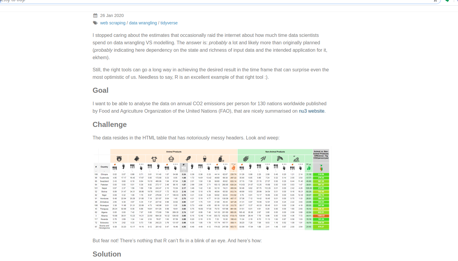
ScreenShot
Animal vs. Non-Animal CO2
These data will require some recreation; that’s the reason for keeping and creating the wide data above. The pivots. I don’t really care so much about the actual food production here; this is about the carbon footprint. There is a color coding key to the above spreadsheet and I just need to pull it out. The oranges are animal and the greens are not. Just pick out the right columns to sum up and we are ready to go. Above, that is the FCC02W data.frame. As an aside, this is yet another criticism of spreadsheets; you can encode data in the colors that isn’t recoverable in any interesting way.
First, the reason they are missing is that that part of the scraping is a bit kludgy; the original author was seeking comment on it. Perhaps you can skip columns that are sums of those that precede it. The tidyTuesday has the cleaning script. I just have to remove the filter.
library(tidyverse)
library(janitor)
##
## Attaching package: 'janitor'## The following objects are masked from 'package:stats':
##
## chisq.test, fisher.testlibrary(rvest)## Loading required package: xml2##
## Attaching package: 'rvest'## The following object is masked from 'package:purrr':
##
## pluck## The following object is masked from 'package:readr':
##
## guess_encoding# Credit to Kasia and minorly edited to create output file and test plot
# Blog post at https://r-tastic.co.uk/post/from-messy-to-tidy/
url <- "https://www.nu3.de/blogs/nutrition/food-carbon-footprint-index-2018"
# scrape the website
url_html <- read_html(url)
# extract the HTML table
whole_table <- url_html %>%
html_nodes('table') %>%
html_table(fill = TRUE) %>%
.[[1]]
table_content <- whole_table %>%
select(-X1) %>% # remove redundant column
filter(!dplyr::row_number() %in% 1:3) # remove redundant rows
raw_headers <- url_html %>%
html_nodes(".thead-icon") %>%
html_attr('title')
tidy_bottom_header <- raw_headers[28:length(raw_headers)]
tidy_bottom_header[1:10]## [1] "Supplied for Consumption (kg/person/year)"
## [2] "Kg CO2/person/year"
## [3] "Supplied for Consumption (kg/person/year)"
## [4] "Kg CO2/person/year"
## [5] "Supplied for Consumption (kg/person/year)"
## [6] "Kg CO2/person/year"
## [7] "Supplied for Consumption (kg/person/year)"
## [8] "Kg CO2/person/year"
## [9] "Supplied for Consumption (kg/person/year)"
## [10] "Kg CO2/person/year"raw_middle_header <- raw_headers[17:27]
raw_middle_header## [1] "Pork" "Poultry"
## [3] "Beef" "Lamb & Goat"
## [5] "Fish" "Eggs"
## [7] "Milk - inc. cheese" "Wheat and Wheat Products"
## [9] "Rice" "Soybeans"
## [11] "Nuts inc. Peanut Butter"tidy_headers <- c(
rep(raw_middle_header[1:7], each = 2),
"animal_total",
rep(raw_middle_header[8:length(raw_middle_header)], each = 2),
"non_animal_total",
"country_total")
tidy_headers## [1] "Pork" "Pork"
## [3] "Poultry" "Poultry"
## [5] "Beef" "Beef"
## [7] "Lamb & Goat" "Lamb & Goat"
## [9] "Fish" "Fish"
## [11] "Eggs" "Eggs"
## [13] "Milk - inc. cheese" "Milk - inc. cheese"
## [15] "animal_total" "Wheat and Wheat Products"
## [17] "Wheat and Wheat Products" "Rice"
## [19] "Rice" "Soybeans"
## [21] "Soybeans" "Nuts inc. Peanut Butter"
## [23] "Nuts inc. Peanut Butter" "non_animal_total"
## [25] "country_total"combined_colnames <- paste(tidy_headers, tidy_bottom_header, sep = ';')
colnames(table_content) <- c("Country", combined_colnames)
glimpse(table_content[, 1:10])## Observations: 130
## Variables: 10
## $ Country <chr> "Argentina", …
## $ `Pork;Supplied for Consumption (kg/person/year)` <chr> "10.51", "24.…
## $ `Pork;Kg CO2/person/year` <chr> "37.20", "85.…
## $ `Poultry;Supplied for Consumption (kg/person/year)` <chr> "38.66", "46.…
## $ `Poultry;Kg CO2/person/year` <chr> "41.53", "49.…
## $ `Beef;Supplied for Consumption (kg/person/year)` <chr> "55.48", "33.…
## $ `Beef;Kg CO2/person/year` <chr> "1712.00", "1…
## $ `Lamb & Goat;Supplied for Consumption (kg/person/year)` <chr> "1.56", "9.87…
## $ `Lamb & Goat;Kg CO2/person/year` <chr> "54.63", "345…
## $ `Fish;Supplied for Consumption (kg/person/year)` <chr> "4.36", "17.6…long_table <- table_content %>%
# make column names observations of Category variable
tidyr::pivot_longer(cols = -Country, names_to = "Category", values_to = "Values") %>%
# separate food-related information from the metric
tidyr::separate(col = Category, into = c("Food Category", "Metric"), sep = ';')
glimpse(long_table)## Observations: 3,250
## Variables: 4
## $ Country <chr> "Argentina", "Argentina", "Argentina", "Argentina", "…
## $ `Food Category` <chr> "Pork", "Pork", "Poultry", "Poultry", "Beef", "Beef",…
## $ Metric <chr> "Supplied for Consumption (kg/person/year)", "Kg CO2/…
## $ Values <chr> "10.51", "37.20", "38.66", "41.53", "55.48", "1712.00…tidy_table <- long_table %>%
tidyr::pivot_wider(names_from = Metric, values_from = Values) %>%
janitor::clean_names('snake')
glimpse(tidy_table)## Observations: 1,820
## Variables: 4
## $ country <chr> "Argentina", "Argentina", "Ar…
## $ food_category <chr> "Pork", "Poultry", "Beef", "L…
## $ supplied_for_consumption_kg_person_year <chr> "10.51", "38.66", "55.48", "1…
## $ kg_co2_person_year <chr> "37.20", "41.53", "1712.00", …final_table <- tidy_table %>%
rename(consumption = 3,
co2_emission = 4)
clean_table <- final_table %>%
mutate_at(vars(consumption, co2_emission), parse_number)An Alternative
Quick and dirty base R.
names(FCCO2W)## [1] "country" "CO2_Pork"
## [3] "CO2_Poultry" "CO2_Beef"
## [5] "CO2_Lamb & Goat" "CO2_Fish"
## [7] "CO2_Eggs" "CO2_Milk - inc. cheese"
## [9] "CO2_Wheat and Wheat Products" "CO2_Rice"
## [11] "CO2_Soybeans" "CO2_Nuts inc. Peanut Butter"
## [13] "CO2_Total"FCCO2W$Animal.CO2 <- rowSums(FCCO2W[,c(2:8)])
FCCO2W$Non.Animal.CO2 <- rowSums(FCCO2W[,c(9:12)])
FCC02W <- FCCO2W %>% mutate(CO2.Footprint.Difference = Animal.CO2 - Non.Animal.CO2)And plot it.
FCWM <- world_map %>% left_join(., FCC02W)## Joining, by = "country"WMCO2 <- ggplot(FCWM, aes(x = long, y = lat, group = group, fill=CO2_Total)) +
geom_polygon(colour = "white") +
scale_fill_viridis_c(option = "B") +
labs(fill = "CO2 kg/person/yr", title="CO2 Difference (Animal - Non-Animal)", subtitle ="from Food Produced for Consumption", caption="a #tidyTuesday by @PieRatio")
WMCO2