Trump's Tweets, Part II
Trump’s Tone
A cool post on sentiment analysis can be found here. I will now get at the time series characteristics of his tweets and the sentiment stuff. This plays off of a previous post.
I start by loading the tmls object that I created in the previous post. To capture constant content over time, there I describe how to download and break up the timeline.
Trump’s Overall Tweeting
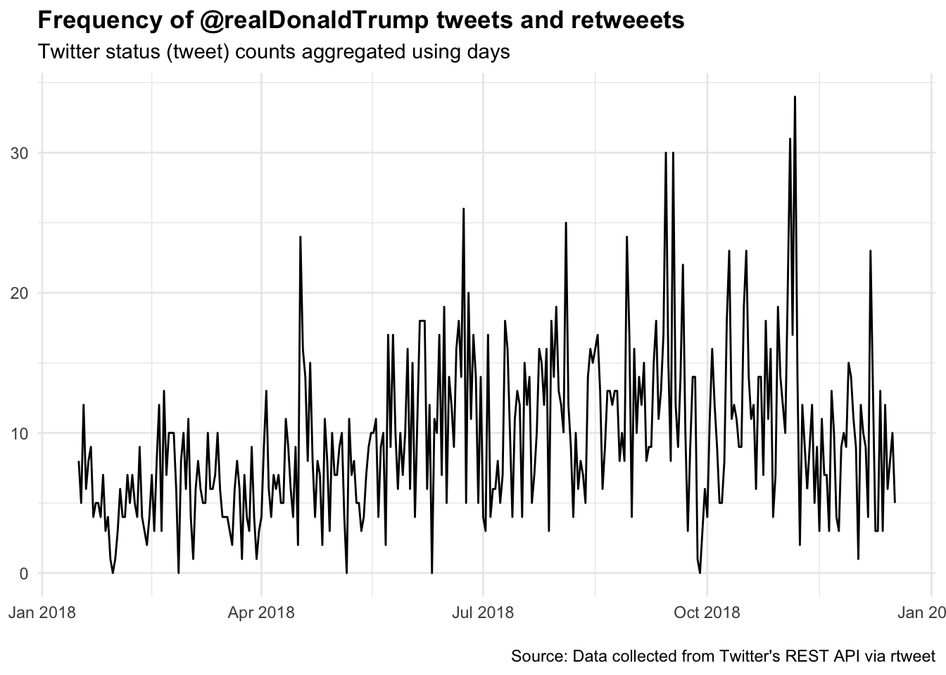
What does it look like?
library(tidyverse)
library(tidytext)
library(SnowballC)
library(tm)
library(syuzhet)
library(rtweet)
load(url("https://github.com/robertwwalker/academic-mymod/raw/master/data/TMLS.RData"))
names(tml.djt)
## [1] "user_id" "status_id"
## [3] "created_at" "screen_name"
## [5] "text" "source"
## [7] "display_text_width" "reply_to_status_id"
## [9] "reply_to_user_id" "reply_to_screen_name"
## [11] "is_quote" "is_retweet"
## [13] "favorite_count" "retweet_count"
## [15] "hashtags" "symbols"
## [17] "urls_url" "urls_t.co"
## [19] "urls_expanded_url" "media_url"
## [21] "media_t.co" "media_expanded_url"
## [23] "media_type" "ext_media_url"
## [25] "ext_media_t.co" "ext_media_expanded_url"
## [27] "ext_media_type" "mentions_user_id"
## [29] "mentions_screen_name" "lang"
## [31] "quoted_status_id" "quoted_text"
## [33] "quoted_created_at" "quoted_source"
## [35] "quoted_favorite_count" "quoted_retweet_count"
## [37] "quoted_user_id" "quoted_screen_name"
## [39] "quoted_name" "quoted_followers_count"
## [41] "quoted_friends_count" "quoted_statuses_count"
## [43] "quoted_location" "quoted_description"
## [45] "quoted_verified" "retweet_status_id"
## [47] "retweet_text" "retweet_created_at"
## [49] "retweet_source" "retweet_favorite_count"
## [51] "retweet_retweet_count" "retweet_user_id"
## [53] "retweet_screen_name" "retweet_name"
## [55] "retweet_followers_count" "retweet_friends_count"
## [57] "retweet_statuses_count" "retweet_location"
## [59] "retweet_description" "retweet_verified"
## [61] "place_url" "place_name"
## [63] "place_full_name" "place_type"
## [65] "country" "country_code"
## [67] "geo_coords" "coords_coords"
## [69] "bbox_coords" "status_url"
## [71] "name" "location"
## [73] "description" "url"
## [75] "protected" "followers_count"
## [77] "friends_count" "listed_count"
## [79] "statuses_count" "favourites_count"
## [81] "account_created_at" "verified"
## [83] "profile_url" "profile_expanded_url"
## [85] "account_lang" "profile_banner_url"
## [87] "profile_background_url" "profile_image_url"ts_plot(tml.djt, "days") +
ggplot2::theme_minimal() +
ggplot2::theme(plot.title = ggplot2::element_text(face = "bold")) +
ggplot2::labs(
x = NULL, y = NULL,
title = "Frequency of @realDonaldTrump tweets and retweeets",
subtitle = "Twitter status (tweet) counts aggregated using days",
caption = "\nSource: Data collected from Twitter's REST API via rtweet"
)
Trump’s Tweets by Day
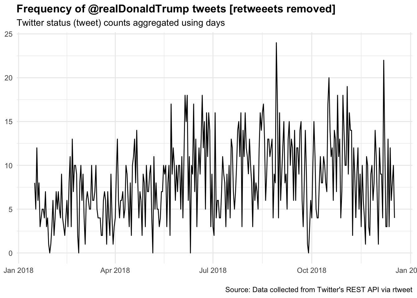
I want to first get rid of retweets to render President Trump in his own voice.
DJTDF <- tml.djt %>% filter(is_retweet==FALSE)
ts_plot(DJTDF, "days") +
  ggplot2::theme_minimal() +
  ggplot2::theme(plot.title = ggplot2::element_text(face = "bold")) +
  ggplot2::labs(
    x = NULL, y = NULL,
    title = "Frequency of @realDonaldTrump tweets [retweeets removed]",
    subtitle = "Twitter status (tweet) counts aggregated using days",
    caption = "\nSource: Data collected from Twitter's REST API via rtweet"
  )
Some more stuff from stack overflow. There is quite a bit of code in here. I simply wrote a function that takes an input character string and cleans it up. Uncomment the various components and pipe them. The sequencing is important and I found this to get everything that I wanted.
library(RColorBrewer)
TDF <- DJTDF %>% select(text)
library(tidyr)
CT <- TDF %>% mutate(tweetno= row_number())
# TDF contains the text of tweets amd the id
library(stringr)
tweet_cleaner <- function(text) {
temp1 <- str_replace_all(text, "&", "") %>%
str_replace_all(., "https.*","") %>%
# str_replace_all(., "http.*", "") %>%
str_replace_all(.,"@[a-z,A-Z]*","")
# str_replace_all(., "[[:punct:]]", "")
# str_replace_all(., "[[:digit:]]", "") %>%
# str_replace_all(., "[ \t]{2,}", "") %>%
# str_replace_all(., "^\\s+|\\s+$", "") %>%
# str_replace_all(., " "," ") %>%
# str_replace_all(.,"RT @[a-z,A-Z]*: ","") %>%
# str_replace_all(.,"#[a-z,A-Z]*","")
return(temp1)
}
clean_tweets <- data.frame(text=sapply(1:dim(TDF)[[1]], function(x) {tweet_cleaner(TDF[x,"text"])}))
clean_tweets$text <- as.character(clean_tweets$text)
clean_tweets$created_at <- DJTDF$created_at
Trumps.Sent.Words <- clean_tweets %>% unnest_tokens(., word, text) %>% anti_join(stop_words, "word")
# word.df <- as.vector(TDF)
# emotion.df <- get_nrc_sentiment(word.df)
SNTR1 <- apply(TDF, 1, function(x) {get_nrc_sentiment(x)})
Sent.Res <- bind_rows(SNTR1)
head(Sent.Res)## anger anticipation disgust fear joy sadness surprise trust negative
## text...1 1 1 0 2 2 0 1 4 3
## text...2 0 2 0 0 2 0 1 2 0
## text...3 0 1 0 1 1 0 0 1 1
## text...4 1 1 0 1 0 1 1 0 1
## text...5 4 1 4 3 0 3 1 1 4
## text...6 3 0 4 2 0 3 1 1 4
## positive
## text...1 4
## text...2 3
## text...3 2
## text...4 3
## text...5 0
## text...6 1A Single Number Sentiment
library(tidytext)
SNTRB <- apply(TDF, 1, function(x) {get_sentiment(x, method="bing")})
DJTDF$Bing <- SNTRB
DJTDF <- DJTDF %>% mutate(RN=row_number())
DJTDF <- DJTDF
DJTDF <- DJTDF[order(DJTDF$RN, decreasing = T),]
library(tibbletime)
##
## Attaching package: 'tibbletime'## The following object is masked from 'package:stats':
##
## filterDJTDF_tbl_time_d <- DJTDF %>%
as_tbl_time(index = created_at)
My.Res <- DJTDF_tbl_time_d %>%
collapse_by("daily") %>%
dplyr::group_by(created_at) %>%
dplyr::summarise_if(is.numeric, mean) %>% select(created_at,Bing)
SBP <- My.Res %>% filter(Bing>0)
SBN <- My.Res %>% filter(Bing<0)
plot(My.Res, type="l", xlab="2018", ylab="Avg. Bing Sentiment", main="Trump's Bing Daily Mood")
points(SBP, col="green")
points(SBN, col="red")
text(My.Res[316,], "GHW Bush Passes", cex=0.6)
text(My.Res[66,], "March for Our Life", cex=0.6)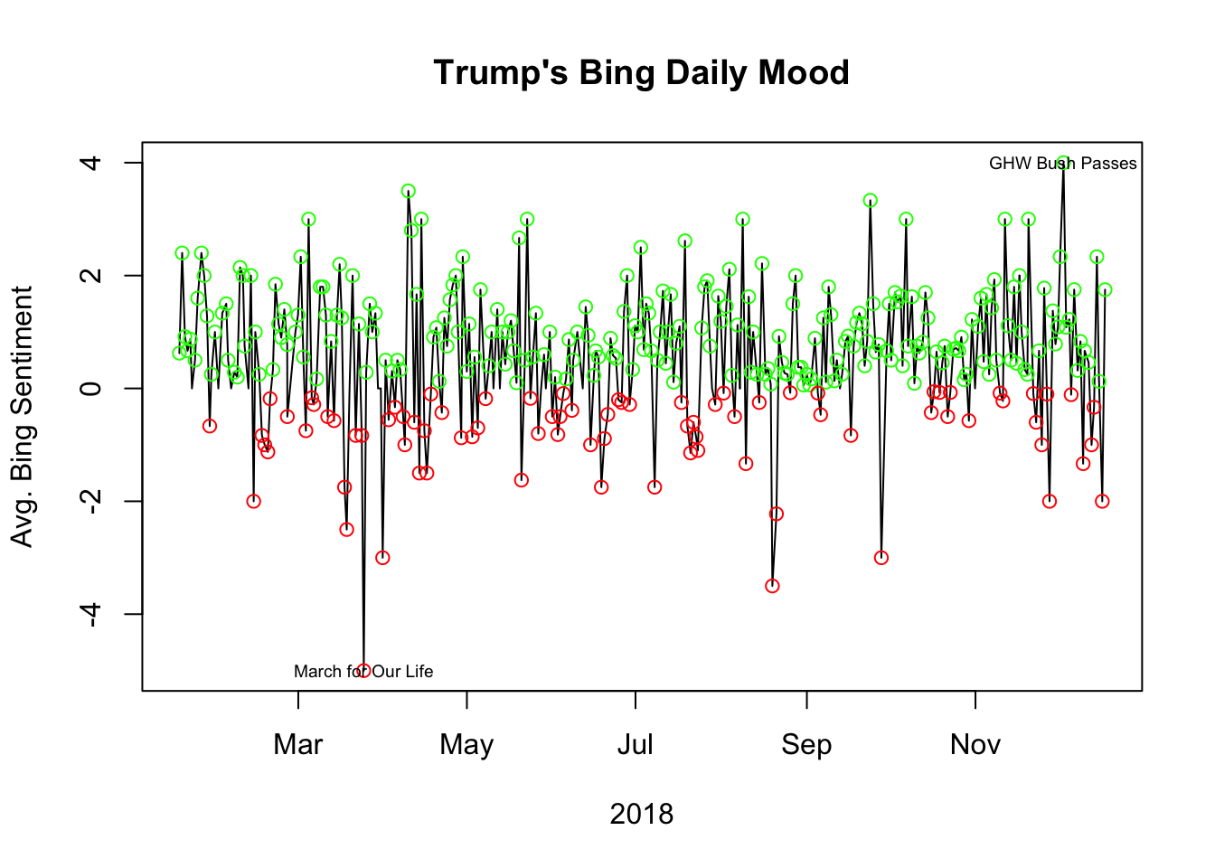
table(sign(My.Res$Bing))##
## -1 0 1
## 84 16 231That’s pretty interesting. There are considerably more positive days than negative ones. The timing of the maximum and minimum are fairly clear in time. Some changes the tidytext and licenses for sentiments broke this. To fix it, I have to save a local.
tidy.tweets <- DJTDF %>% select(created_at, text) %>% unnest_tokens(word, text)
afinn <- tidy.tweets %>%
  inner_join(get_sentiments("afinn")) %>%
  group_by(created_at) %>%
  summarise(sentiment = sum(value)) %>%
  mutate(method = "AFINN")
bing_and_nrc <- bind_rows(tidy.tweets %>%
                            inner_join(get_sentiments("bing")) %>%
                            mutate(method = "Bing"),
                          tidy.tweets %>%
                            inner_join(get_sentiments("nrc") %>%
                                         filter(sentiment %in% c("positive",
                                                                 "negative"))) %>%
                            mutate(method = "NRC")) %>%
  count(method, created_at, sentiment) %>%
  spread(sentiment, n, fill = 0) %>%
  mutate(sentiment = positive - negative) %>% select(created_at, sentiment, method)
Sents.Me <- bind_rows(afinn,bing_and_nrc)
SME_tbl_time_d <- Sents.Me  %>% as_tbl_time(index = created_at)
My.Res <- SME_tbl_time_d %>% group_by(method) %>%
    collapse_by("daily") %>%
    dplyr::group_by(created_at, method) %>%
    dplyr::summarise_if(is.numeric, mean) %>% ungroup()
save(Sents.Me,SME_tbl_time_d,My.Res,bing_and_nrc,tidy.tweets, file="~/TrumpTweets.RData")
load("TrumpTweets.RData")
ggplot(data = My.Res) +
aes(x = created_at, y = sentiment, color = method) +
geom_line() +
theme_minimal()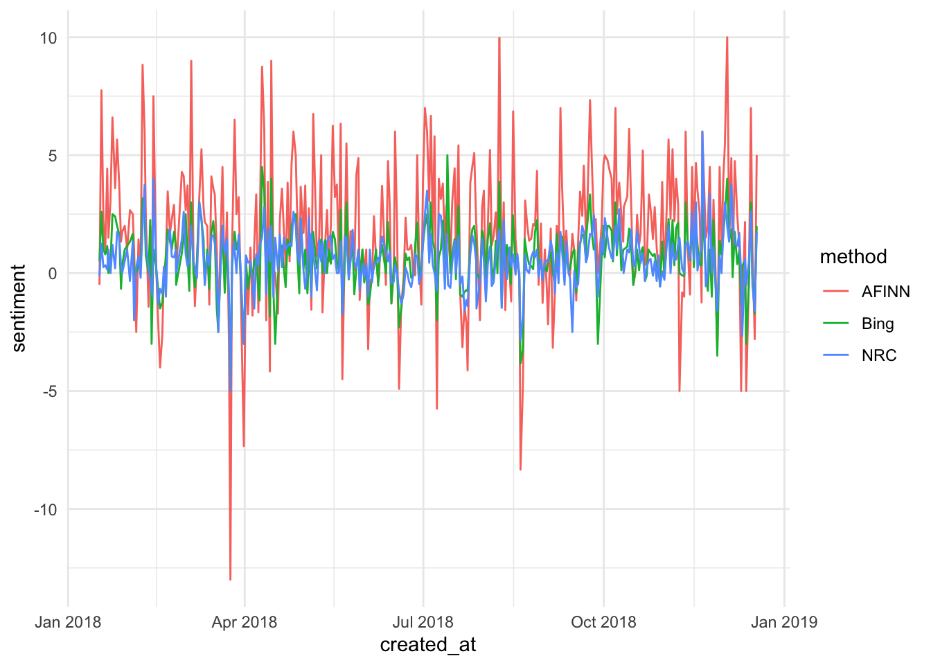
Averaging three types of scaled sentiments
MRS <- My.Res %>% group_by(method) %>% mutate(SS=scale(sentiment))
MRS2 <- MRS %>%  collapse_by("daily") %>% select(created_at, SS) %>%
    dplyr::group_by(created_at) %>%
    dplyr::summarise_if(is.numeric, mean)
## Adding missing grouping variables: `method`ggplot(data = MRS2) +
aes(x = created_at, y = SS) +
geom_line(color = '#781c6d') +
labs(title = 'Sentiment: Averaged',
x = 'Date',
y = 'Mean Scaled Sentiment') +
theme_minimal()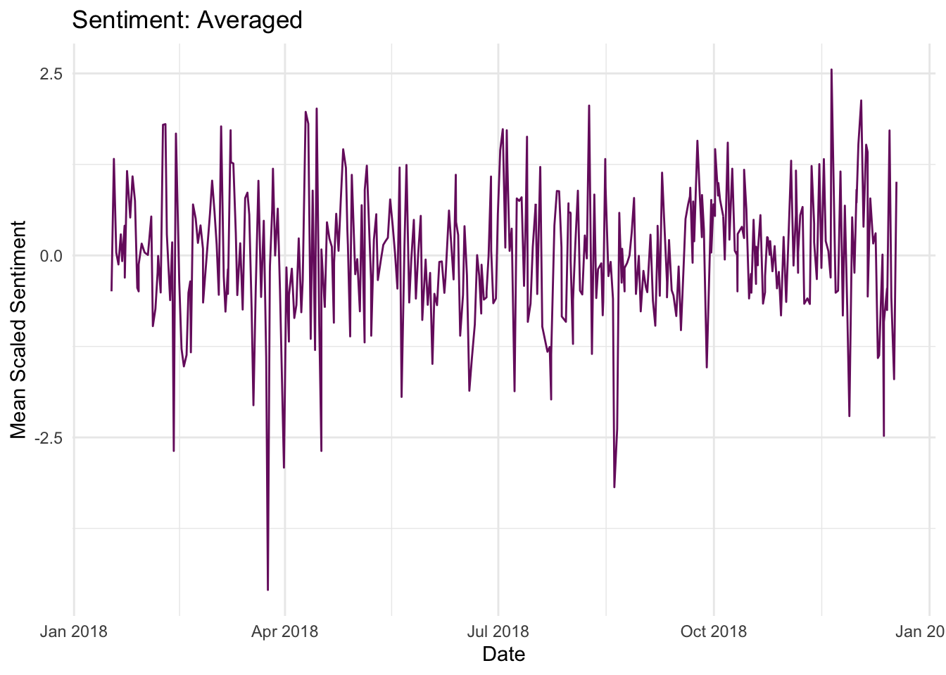
Common Words
The comparson_cloud() features in wordcloud allow a split of the most common words in the positive and negative sentiment dictionaries.
library(wordcloud)
library(reshape2)
##
## Attaching package: 'reshape2'## The following object is masked from 'package:tidyr':
##
## smithstidy.tweets %>%
inner_join(get_sentiments("bing")) %>%
count(word, sentiment, sort = TRUE) %>%
acast(word ~ sentiment, value.var = "n", fill = 0) %>%
comparison.cloud(colors = c("red","green"),
max.words = 100)## Joining, by = "word"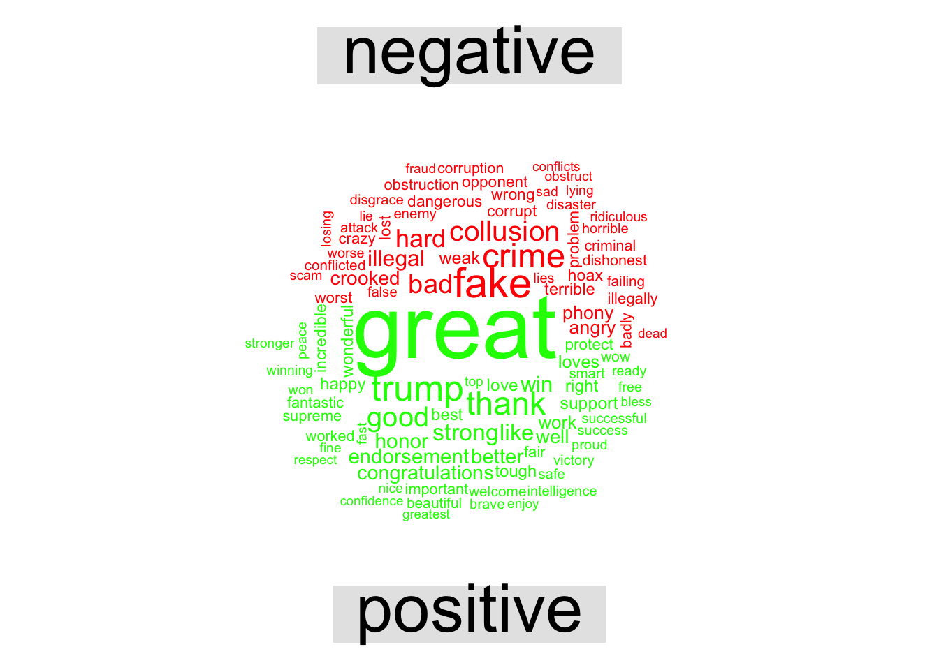
Networks
library(dplyr)
library(tidyr)
library(tidytext)
library(ggplot2)
library(igraph)
##
## Attaching package: 'igraph'## The following objects are masked from 'package:dplyr':
##
## as_data_frame, groups, union## The following objects are masked from 'package:purrr':
##
## compose, simplify## The following object is masked from 'package:tidyr':
##
## crossing## The following object is masked from 'package:tibble':
##
## as_data_frame## The following objects are masked from 'package:stats':
##
## decompose, spectrum## The following object is masked from 'package:base':
##
## unionlibrary(ggraph)
count_bigrams <- function(dataset) {
dataset %>%
unnest_tokens(bigram, text, token = "ngrams", n = 2) %>%
separate(bigram, c("word1", "word2"), sep = " ") %>%
filter(!word1 %in% stop_words$word,
!word2 %in% stop_words$word) %>%
count(word1, word2, sort = TRUE)
}
visualize_bigrams <- function(bigrams) {
set.seed(2016)
a <- grid::arrow(type = "closed", length = unit(.15, "inches"))
bigrams %>%
graph_from_data_frame() %>%
ggraph(layout = "fr") +
geom_edge_link(aes(edge_alpha = n), show.legend = FALSE, arrow = a) +
geom_node_point(color = "lightblue", size = 5) +
geom_node_text(aes(label = name), vjust = 1, hjust = 1) +
theme_void()
}
library(stringr)
djt_bigrams <- clean_tweets %>% select(created_at, text) %>%
count_bigrams()
# filter out rare combinations, as well as digits
djt_bigrams %>%
filter(n > 20,
!str_detect(word1, "\\d"),
!str_detect(word2, "\\d")) %>%
visualize_bigrams()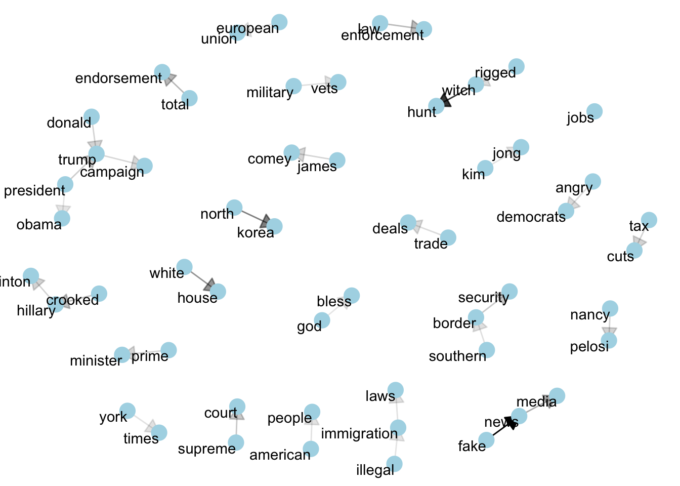
clean_tweets$RN <- DJTDF$RN
tidy.tweets.RN <- clean_tweets %>% select(RN, text) %>% unnest_tokens(word, text) %>%
  anti_join(stop_words) %>%
  count(RN, word, sort = TRUE) %>%
  ungroup()
## Joining, by = "word"tweets_dtm <- tidy.tweets.RN %>%
cast_dtm(RN, word, n)
library(topicmodels)
tweets_lda <- LDA(tweets_dtm, k = 7, control = list(seed = 12345))
tweet_topics <- tidy(tweets_lda, matrix="beta")
top_terms <- tweet_topics %>% group_by(topic) %>% top_n(10, beta) %>%
ungroup() %>%
arrange(topic, -beta)
top_terms %>%
mutate(term = reorder(term, beta)) %>%
ggplot(aes(term, beta, fill = factor(topic))) +
geom_col(show.legend = FALSE) +
facet_wrap(~ topic, scales = "free") +
coord_flip()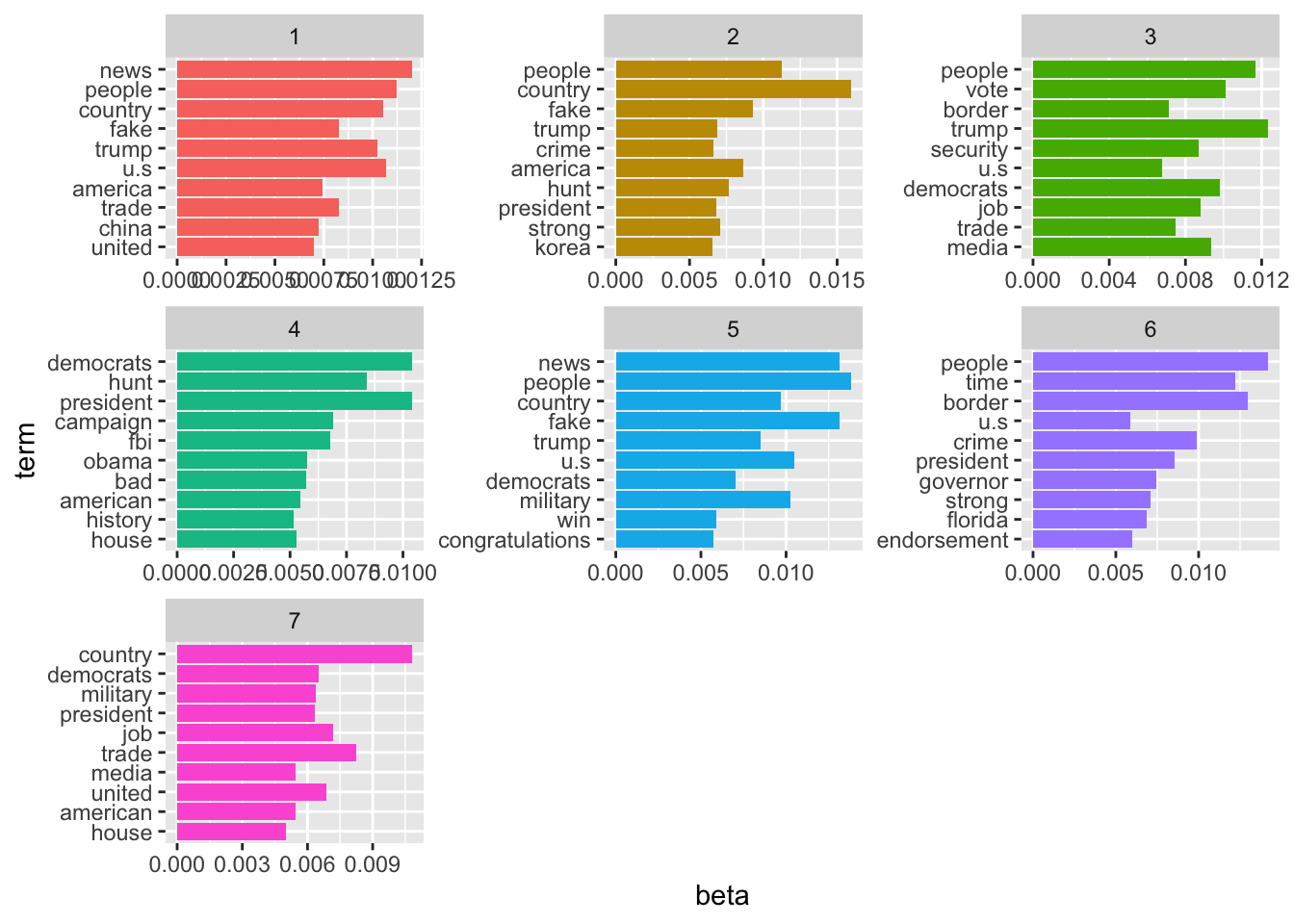
tweet_topicM <- tidy(tweets_lda, matrix="gamma")
top_tweets <- tweet_topicM %>% group_by(topic) %>% top_n(10, gamma) %>%
    ungroup() %>%
    arrange(topic, -gamma)
top_tweets
## # A tibble: 70 x 3
## document topic gamma
## <chr> <int> <dbl>
## 1 1888 1 0.172
## 2 555 1 0.171
## 3 252 1 0.170
## 4 234 1 0.167
## 5 1830 1 0.166
## 6 1340 1 0.166
## 7 2525 1 0.166
## 8 434 1 0.163
## 9 1101 1 0.162
## 10 399 1 0.162
## # … with 60 more rowsTweet.Res <- cbind(TDF[as.numeric(top_tweets$document),],top_tweets)Mallet is finicky. Below is some playing with it but the stop words are messy.
library(qdap)
clean_tweets$text <- clean_tweets %>% select(text) %>% rm_stopwords(., tm::stopwords("english"), separate = FALSE, unlist=FALSE)
library(mallet)
clean_tweets$RN <- as.character(clean_tweets$RN)
clean_tweets <- clean_tweets
# create an empty file of "stopwords"
# file.create(empty_file <- tempfile())
# mystopwords <- as.character(stop_words[,1])
stopwords_en <-  stop_words
#system.file("stoplists/en.txt", package = "mallet")
docs <- mallet.import(clean_tweets$RN, clean_tweets$text, stoplist=stopwords_en)
mallet_model <- MalletLDA(num.topics = 6)
mallet_model$loadDocuments(docs)
mallet_model$train(250)
mallet_model$maximize(100)
topic.words <- mallet.topic.words(mallet_model, smoothed=TRUE, normalized=TRUE)
names(topic.words)
mallet.top.words(mallet_model, word.weights = topic.words[4,], num.top.words = 5)
Sentiments and Tidy Calendars
Now I want to play with the time series properties of the tweet sentiments. Days of the week and times of day aggregated over different periods can say something… Perhaps some day?