Visualisation with Archigos: Leaders of the World
Archigos
Is an amazing collaboration that produced a comprehensive dataset of world leaders going pretty far back; see Archigos on the web. For thinking about leadership, it is quite natural. In this post, I want to do some reshaping into country year and leader year datasets and explore the basic confines of Archigos. I also want to use gganimate for a few things. So what do we know?
library(lubridate)
library(tidyverse)
library(ggthemes)
library(stringr)
library(gganimate)
library(emoGG)
library(emojifont)
library(haven)
Archigos <- read_dta(url("http://www.rochester.edu/college/faculty/hgoemans/Archigos_4.1_stata14.dta"))
head(Archigos)
## # A tibble: 6 x 28
## obsid leadid ccode idacr leader startdate eindate enddate eoutdate entry
## <chr> <chr> <dbl> <chr> <chr> <chr> <date> <chr> <date> <chr>
## 1 USA-… 81dcc… 2 USA Grant 1869-03-… 1869-03-04 1877-0… 1877-03-04 Regu…
## 2 USA-… 81dcc… 2 USA Hayes 1877-03-… 1877-03-04 1881-0… 1881-03-04 Regu…
## 3 USA-… 81dcf… 2 USA Garfi… 1881-03-… 1881-03-04 1881-0… 1881-09-19 Regu…
## 4 USA-… 81dcf… 2 USA Arthur 1881-09-… 1881-09-19 1885-0… 1885-03-04 Regu…
## 5 USA-… 34fb1… 2 USA Cleve… 1885-03-… 1885-03-04 1889-0… 1889-03-04 Regu…
## 6 USA-… 81dcf… 2 USA Harri… 1889-03-… 1889-03-04 1893-0… 1893-03-04 Regu…
## # … with 18 more variables: exit <chr>, exitcode <chr>,
## # prevtimesinoffice <dbl>, posttenurefate <chr>, gender <chr>, yrborn <dbl>,
## # yrdied <dbl>, borndate <chr>, ebirthdate <date>, deathdate <chr>,
## # edeathdate <date>, dbpediauri <chr>, numentry <dbl>, numexit <dbl>,
## # numexitcode <dbl>, numposttenurefate <dbl>, fties <chr>, ftcur <chr>That’s a pretty impressive span of leaders. Let me obtain a list of the countries. This is a link from the Archigos website to the work of Gleditsch and Ward. The dates that they store are colon rather than dash separated so that needs to be fixed, then I convert the dates to valid date format. There is also a problem with the text encoding [at least on this Linux workstation] for the Ivory Coast. I suspect it is an accent mark.
History of Countries: Gleditsch and Ward
iisystem <- read.delim(url("http://www.ksgleditsch.com/data/iisystem.dat"), col.names=c("ccode","idacr","CountryName","startD","endD"), stringsAsFactors = FALSE)
iisystem <- iisystem %>% mutate(startD = str_replace_all(startD, ":", "-"))
iisystem <- iisystem %>% mutate(endD = str_replace_all(endD, ":", "-"))
iisystem$CountryName[[108]] <- "Ivory Coast"
iisystem$startD <- as_date(dmy(iisystem$startD))
iisystem$endD <- as_date(dmy(iisystem$endD))
iisystem <- iisystem %>% mutate(IISstartYear = year(startD), IISendYear = year(endD))
Some Data Management
There are two datasets that I will want to create to use to analyse this. I am likely to want a dataset of country years and a dataset of leader years. After putting these together, I note that there is actually only one leader that leads two distinct country codes. I am putting this code at the top because others may find it useful.
Country Years
I want to create all valid years for each of the countries identified by the Gleditsch and Ward set of countries. This is a bit of a hack using apply and dimensions but it works. Basically, here is the idea. Use lapply over a list that is just a sequence of row length and apply a function. A row number is the input to the function, create a temporary named vector to operate on in tempd and create a data.frame to pass back with the appropriate sequence of years between the start and end years along with some useful identifiers. The result is a list. To collapse the list, do.call and rbind – binding the rows – do the trick. One can left join them (the result and iisystem) back together as a sanity check.
# Build a grid of countries and years
DI <- as.integer(dim(iisystem)[[1]])
tseq <-function(x) {
tempd <- iisystem[x,]
data.frame(ccode = tempd$ccode, CountryName = as.character(tempd$CountryName), idacr=as.character(tempd$idacr), year=seq(tempd$IISstartYear, tempd$IISendYear, by=1), IISstartYear = tempd$IISstartYear, IISendYear = tempd$IISendYear, startD = tempd$startD, endD = tempd$endD)
}
CSTS <- lapply(seq(1,DI), function(x) { tseq(x) } )
CSTS.Data <- data.frame(do.call(rbind, CSTS))
CSTS.Data$CountryName <- as.character(CSTS.Data$CountryName)
CSTS.Data$idacr <- as.character(CSTS.Data$idacr)
# That gets it.  Down to nt=17565.
CSTS.Data is my result. It has been saved in a subdirectory Archigos-etc of my data on GitHub. You can load it with:
CSTS.Data <- readRDS(url("https://github.com/robertwwalker/academic-mymod/raw/master/data/Archigos-etc/GWCSTS.rds"))
CSTS.Data <- read.csv("https://github.com/robertwwalker/academic-mymod/raw/master/data/Archigos-etc/GWCSTS.csv", stringsAsFactors=FALSE)
Now I want to accomplish the same thing with a dataset of leaders. The unit here is the leader year. Each leader in Archigos will appear at least once. The method is identical.
Archigos <- Archigos %>% group_by(obsid) %>% mutate(startYear = year(startdate), endYear = year(enddate)) %>% ungroup()
Archigos$obsid <- as.character(Archigos$obsid)
DI <- dim(Archigos)[[1]]
tseq <-function(x) {
  tempd <- Archigos[x,]
  data.frame(obsid = tempd$obsid, leader = as.character(tempd$leader), leadid = as.character(tempd$leadid), idacr=as.character(tempd$idacr), year=seq(tempd$startYear, tempd$endYear, by=1), LSY=tempd$startYear, LEY = tempd$endYear)
}
LTS <- lapply(seq(1,DI), function(x) { tseq(x) } )
LTS.Data <- data.frame(do.call(rbind, LTS))
LTS.Data$idacr <- as.character(LTS.Data$idacr)
LTS.Data$obsid <- as.character(LTS.Data$obsid)
Archigos$obsid <- as.character(Archigos$obsid)
Full.LTS <- LTS.Data %>% left_join(Archigos, by=c("obsid" = "obsid"))
# One curiosity; does any leader lead two distinct countries?  Having the ccodes allows me to calculate the standard deviation by leader.
Full.LTS %>% group_by(leadid.x) %>% summarise(CC.sd = sd(ccode)) %>% arrange(desc(CC.sd)) %>% filter(CC.sd > 0)
## # A tibble: 2 x 2
## leadid.x CC.sd
## <chr> <dbl>
## 1 81de4823-1e42-11e4-b4cd-db5882bf8def 6.93
## 2 821be4de-1e42-11e4-b4cd-db5882bf8def 2.67# If countries are a proper nesting operator, then things can be made much easier. They
Full.LTS %>% filter(leadid.x == "81de4823-1e42-11e4-b4cd-db5882bf8def") # This one seems to be an error with implications## obsid leader.x leadid.x idacr.x
## 1 CAN-1921 King 81de4823-1e42-11e4-b4cd-db5882bf8def CAN
## 2 CAN-1921 King 81de4823-1e42-11e4-b4cd-db5882bf8def CAN
## 3 CAN-1921 King 81de4823-1e42-11e4-b4cd-db5882bf8def CAN
## 4 CAN-1921 King 81de4823-1e42-11e4-b4cd-db5882bf8def CAN
## 5 CAN-1921 King 81de4823-1e42-11e4-b4cd-db5882bf8def CAN
## 6 CAN-1921 King 81de4823-1e42-11e4-b4cd-db5882bf8def CAN
## 7 CAN-1926-2 King 81de4823-1e42-11e4-b4cd-db5882bf8def CAN
## 8 CAN-1926-2 King 81de4823-1e42-11e4-b4cd-db5882bf8def CAN
## 9 CAN-1926-2 King 81de4823-1e42-11e4-b4cd-db5882bf8def CAN
## 10 CAN-1926-2 King 81de4823-1e42-11e4-b4cd-db5882bf8def CAN
## 11 CAN-1926-2 King 81de4823-1e42-11e4-b4cd-db5882bf8def CAN
## 12 CAN-1935 King 81de4823-1e42-11e4-b4cd-db5882bf8def CAN
## 13 CAN-1935 King 81de4823-1e42-11e4-b4cd-db5882bf8def CAN
## 14 CAN-1935 King 81de4823-1e42-11e4-b4cd-db5882bf8def CAN
## 15 CAN-1935 King 81de4823-1e42-11e4-b4cd-db5882bf8def CAN
## 16 CAN-1935 King 81de4823-1e42-11e4-b4cd-db5882bf8def CAN
## 17 CAN-1935 King 81de4823-1e42-11e4-b4cd-db5882bf8def CAN
## 18 CAN-1935 King 81de4823-1e42-11e4-b4cd-db5882bf8def CAN
## 19 CAN-1935 King 81de4823-1e42-11e4-b4cd-db5882bf8def CAN
## 20 CAN-1935 King 81de4823-1e42-11e4-b4cd-db5882bf8def CAN
## 21 CAN-1935 King 81de4823-1e42-11e4-b4cd-db5882bf8def CAN
## 22 CAN-1935 King 81de4823-1e42-11e4-b4cd-db5882bf8def CAN
## 23 CAN-1935 King 81de4823-1e42-11e4-b4cd-db5882bf8def CAN
## 24 CAN-1935 King 81de4823-1e42-11e4-b4cd-db5882bf8def CAN
## 25 CAN-1935 King 81de4823-1e42-11e4-b4cd-db5882bf8def CAN
## 26 DOM-1876-4 Buenaventura Baez 81de4823-1e42-11e4-b4cd-db5882bf8def DOM
## 27 DOM-1876-4 Buenaventura Baez 81de4823-1e42-11e4-b4cd-db5882bf8def DOM
## 28 DOM-1876-4 Buenaventura Baez 81de4823-1e42-11e4-b4cd-db5882bf8def DOM
## year LSY LEY leadid.y ccode idacr.y
## 1 1921 1921 1926 81de4823-1e42-11e4-b4cd-db5882bf8def 20 CAN
## 2 1922 1921 1926 81de4823-1e42-11e4-b4cd-db5882bf8def 20 CAN
## 3 1923 1921 1926 81de4823-1e42-11e4-b4cd-db5882bf8def 20 CAN
## 4 1924 1921 1926 81de4823-1e42-11e4-b4cd-db5882bf8def 20 CAN
## 5 1925 1921 1926 81de4823-1e42-11e4-b4cd-db5882bf8def 20 CAN
## 6 1926 1921 1926 81de4823-1e42-11e4-b4cd-db5882bf8def 20 CAN
## 7 1926 1926 1930 81de4823-1e42-11e4-b4cd-db5882bf8def 20 CAN
## 8 1927 1926 1930 81de4823-1e42-11e4-b4cd-db5882bf8def 20 CAN
## 9 1928 1926 1930 81de4823-1e42-11e4-b4cd-db5882bf8def 20 CAN
## 10 1929 1926 1930 81de4823-1e42-11e4-b4cd-db5882bf8def 20 CAN
## 11 1930 1926 1930 81de4823-1e42-11e4-b4cd-db5882bf8def 20 CAN
## 12 1935 1935 1948 81de4823-1e42-11e4-b4cd-db5882bf8def 20 CAN
## 13 1936 1935 1948 81de4823-1e42-11e4-b4cd-db5882bf8def 20 CAN
## 14 1937 1935 1948 81de4823-1e42-11e4-b4cd-db5882bf8def 20 CAN
## 15 1938 1935 1948 81de4823-1e42-11e4-b4cd-db5882bf8def 20 CAN
## 16 1939 1935 1948 81de4823-1e42-11e4-b4cd-db5882bf8def 20 CAN
## 17 1940 1935 1948 81de4823-1e42-11e4-b4cd-db5882bf8def 20 CAN
## 18 1941 1935 1948 81de4823-1e42-11e4-b4cd-db5882bf8def 20 CAN
## 19 1942 1935 1948 81de4823-1e42-11e4-b4cd-db5882bf8def 20 CAN
## 20 1943 1935 1948 81de4823-1e42-11e4-b4cd-db5882bf8def 20 CAN
## 21 1944 1935 1948 81de4823-1e42-11e4-b4cd-db5882bf8def 20 CAN
## 22 1945 1935 1948 81de4823-1e42-11e4-b4cd-db5882bf8def 20 CAN
## 23 1946 1935 1948 81de4823-1e42-11e4-b4cd-db5882bf8def 20 CAN
## 24 1947 1935 1948 81de4823-1e42-11e4-b4cd-db5882bf8def 20 CAN
## 25 1948 1935 1948 81de4823-1e42-11e4-b4cd-db5882bf8def 20 CAN
## 26 1876 1876 1878 81de4823-1e42-11e4-b4cd-db5882bf8def 42 DOM
## 27 1877 1876 1878 81de4823-1e42-11e4-b4cd-db5882bf8def 42 DOM
## 28 1878 1876 1878 81de4823-1e42-11e4-b4cd-db5882bf8def 42 DOM
## leader.y startdate eindate enddate eoutdate entry
## 1 King 1921-12-29 1921-12-29 1926-06-28 1926-06-28 Regular
## 2 King 1921-12-29 1921-12-29 1926-06-28 1926-06-28 Regular
## 3 King 1921-12-29 1921-12-29 1926-06-28 1926-06-28 Regular
## 4 King 1921-12-29 1921-12-29 1926-06-28 1926-06-28 Regular
## 5 King 1921-12-29 1921-12-29 1926-06-28 1926-06-28 Regular
## 6 King 1921-12-29 1921-12-29 1926-06-28 1926-06-28 Regular
## 7 King 1926-09-25 1926-09-25 1930-08-07 1930-08-07 Regular
## 8 King 1926-09-25 1926-09-25 1930-08-07 1930-08-07 Regular
## 9 King 1926-09-25 1926-09-25 1930-08-07 1930-08-07 Regular
## 10 King 1926-09-25 1926-09-25 1930-08-07 1930-08-07 Regular
## 11 King 1926-09-25 1926-09-25 1930-08-07 1930-08-07 Regular
## 12 King 1935-10-23 1935-10-23 1948-11-15 1948-11-15 Regular
## 13 King 1935-10-23 1935-10-23 1948-11-15 1948-11-15 Regular
## 14 King 1935-10-23 1935-10-23 1948-11-15 1948-11-15 Regular
## 15 King 1935-10-23 1935-10-23 1948-11-15 1948-11-15 Regular
## 16 King 1935-10-23 1935-10-23 1948-11-15 1948-11-15 Regular
## 17 King 1935-10-23 1935-10-23 1948-11-15 1948-11-15 Regular
## 18 King 1935-10-23 1935-10-23 1948-11-15 1948-11-15 Regular
## 19 King 1935-10-23 1935-10-23 1948-11-15 1948-11-15 Regular
## 20 King 1935-10-23 1935-10-23 1948-11-15 1948-11-15 Regular
## 21 King 1935-10-23 1935-10-23 1948-11-15 1948-11-15 Regular
## 22 King 1935-10-23 1935-10-23 1948-11-15 1948-11-15 Regular
## 23 King 1935-10-23 1935-10-23 1948-11-15 1948-11-15 Regular
## 24 King 1935-10-23 1935-10-23 1948-11-15 1948-11-15 Regular
## 25 King 1935-10-23 1935-10-23 1948-11-15 1948-11-15 Regular
## 26 Buenaventura Baez 1876-12-26 1876-12-26 1878-03-02 1878-03-02 Irregular
## 27 Buenaventura Baez 1876-12-26 1876-12-26 1878-03-02 1878-03-02 Irregular
## 28 Buenaventura Baez 1876-12-26 1876-12-26 1878-03-02 1878-03-02 Irregular
## exit exitcode prevtimesinoffice posttenurefate gender
## 1 Regular Regular 0 OK M
## 2 Regular Regular 0 OK M
## 3 Regular Regular 0 OK M
## 4 Regular Regular 0 OK M
## 5 Regular Regular 0 OK M
## 6 Regular Regular 0 OK M
## 7 Regular Regular 1 OK M
## 8 Regular Regular 1 OK M
## 9 Regular Regular 1 OK M
## 10 Regular Regular 1 OK M
## 11 Regular Regular 1 OK M
## 12 Retired Due to Ill Health Regular 2 OK M
## 13 Retired Due to Ill Health Regular 2 OK M
## 14 Retired Due to Ill Health Regular 2 OK M
## 15 Retired Due to Ill Health Regular 2 OK M
## 16 Retired Due to Ill Health Regular 2 OK M
## 17 Retired Due to Ill Health Regular 2 OK M
## 18 Retired Due to Ill Health Regular 2 OK M
## 19 Retired Due to Ill Health Regular 2 OK M
## 20 Retired Due to Ill Health Regular 2 OK M
## 21 Retired Due to Ill Health Regular 2 OK M
## 22 Retired Due to Ill Health Regular 2 OK M
## 23 Retired Due to Ill Health Regular 2 OK M
## 24 Retired Due to Ill Health Regular 2 OK M
## 25 Retired Due to Ill Health Regular 2 OK M
## 26 Irregular Unknown 4 Exile M
## 27 Irregular Unknown 4 Exile M
## 28 Irregular Unknown 4 Exile M
## yrborn yrdied borndate ebirthdate deathdate edeathdate
## 1 1874 1951 NA <NA> NA <NA>
## 2 1874 1951 NA <NA> NA <NA>
## 3 1874 1951 NA <NA> NA <NA>
## 4 1874 1951 NA <NA> NA <NA>
## 5 1874 1951 NA <NA> NA <NA>
## 6 1874 1951 NA <NA> NA <NA>
## 7 1874 1951 NA <NA> NA <NA>
## 8 1874 1951 NA <NA> NA <NA>
## 9 1874 1951 NA <NA> NA <NA>
## 10 1874 1951 NA <NA> NA <NA>
## 11 1874 1951 NA <NA> NA <NA>
## 12 1874 1951 NA <NA> NA <NA>
## 13 1874 1951 NA <NA> NA <NA>
## 14 1874 1951 NA <NA> NA <NA>
## 15 1874 1951 NA <NA> NA <NA>
## 16 1874 1951 NA <NA> NA <NA>
## 17 1874 1951 NA <NA> NA <NA>
## 18 1874 1951 NA <NA> NA <NA>
## 19 1874 1951 NA <NA> NA <NA>
## 20 1874 1951 NA <NA> NA <NA>
## 21 1874 1951 NA <NA> NA <NA>
## 22 1874 1951 NA <NA> NA <NA>
## 23 1874 1951 NA <NA> NA <NA>
## 24 1874 1951 NA <NA> NA <NA>
## 25 1874 1951 NA <NA> NA <NA>
## 26 1812 1884 1812-07-14 1812-07-14 1884-03-14 1884-03-14
## 27 1812 1884 1812-07-14 1812-07-14 1884-03-14 1884-03-14
## 28 1812 1884 1812-07-14 1812-07-14 1884-03-14 1884-03-14
## dbpediauri
## 1 NA
## 2 NA
## 3 NA
## 4 NA
## 5 NA
## 6 NA
## 7 NA
## 8 NA
## 9 NA
## 10 NA
## 11 NA
## 12 NA
## 13 NA
## 14 NA
## 15 NA
## 16 NA
## 17 NA
## 18 NA
## 19 NA
## 20 NA
## 21 NA
## 22 NA
## 23 NA
## 24 NA
## 25 NA
## 26 https://urldefense.proofpoint.com/v2/url?u=http-3A__dbpedia.org_resource_Buenaventura-5FB-25C3-25A1ez&d=BQID-g&c=kbmfwr1Yojg42sGEpaQh5ofMHBeTl9EI2eaqQZhHbOU&r=ZliGVSRwfirWoETOrKCh2RSnoygzVPWEk95Me9L-Kwo&m=EaKyFx9mpkhPdFxsxzvW_fiM3jbYwM3xYLjVbSFoDAg&s=BB0NoTztXPjJv_-VzVIsQU7ReKv8HdKXcPFxUvG2w68&e=
## 27 https://urldefense.proofpoint.com/v2/url?u=http-3A__dbpedia.org_resource_Buenaventura-5FB-25C3-25A1ez&d=BQID-g&c=kbmfwr1Yojg42sGEpaQh5ofMHBeTl9EI2eaqQZhHbOU&r=ZliGVSRwfirWoETOrKCh2RSnoygzVPWEk95Me9L-Kwo&m=EaKyFx9mpkhPdFxsxzvW_fiM3jbYwM3xYLjVbSFoDAg&s=BB0NoTztXPjJv_-VzVIsQU7ReKv8HdKXcPFxUvG2w68&e=
## 28 https://urldefense.proofpoint.com/v2/url?u=http-3A__dbpedia.org_resource_Buenaventura-5FB-25C3-25A1ez&d=BQID-g&c=kbmfwr1Yojg42sGEpaQh5ofMHBeTl9EI2eaqQZhHbOU&r=ZliGVSRwfirWoETOrKCh2RSnoygzVPWEk95Me9L-Kwo&m=EaKyFx9mpkhPdFxsxzvW_fiM3jbYwM3xYLjVbSFoDAg&s=BB0NoTztXPjJv_-VzVIsQU7ReKv8HdKXcPFxUvG2w68&e=
## numentry numexit numexitcode numposttenurefate
## 1 0 1.0 0 0
## 2 0 1.0 0 0
## 3 0 1.0 0 0
## 4 0 1.0 0 0
## 5 0 1.0 0 0
## 6 0 1.0 0 0
## 7 0 1.0 0 0
## 8 0 1.0 0 0
## 9 0 1.0 0 0
## 10 0 1.0 0 0
## 11 0 1.0 0 0
## 12 0 2.1 0 0
## 13 0 2.1 0 0
## 14 0 2.1 0 0
## 15 0 2.1 0 0
## 16 0 2.1 0 0
## 17 0 2.1 0 0
## 18 0 2.1 0 0
## 19 0 2.1 0 0
## 20 0 2.1 0 0
## 21 0 2.1 0 0
## 22 0 2.1 0 0
## 23 0 2.1 0 0
## 24 0 2.1 0 0
## 25 0 2.1 0 0
## 26 1 3.0 -999 1
## 27 1 3.0 -999 1
## 28 1 3.0 -999 1
## fties ftcur startYear
## 1 Father of Ramon Baez%81e1556e-1e42-11e4-b4cd-db5882bf8def 1 1921
## 2 Father of Ramon Baez%81e1556e-1e42-11e4-b4cd-db5882bf8def 1 1921
## 3 Father of Ramon Baez%81e1556e-1e42-11e4-b4cd-db5882bf8def 1 1921
## 4 Father of Ramon Baez%81e1556e-1e42-11e4-b4cd-db5882bf8def 1 1921
## 5 Father of Ramon Baez%81e1556e-1e42-11e4-b4cd-db5882bf8def 1 1921
## 6 Father of Ramon Baez%81e1556e-1e42-11e4-b4cd-db5882bf8def 1 1921
## 7 Father of Ramon Baez%81e1556e-1e42-11e4-b4cd-db5882bf8def 1 1926
## 8 Father of Ramon Baez%81e1556e-1e42-11e4-b4cd-db5882bf8def 1 1926
## 9 Father of Ramon Baez%81e1556e-1e42-11e4-b4cd-db5882bf8def 1 1926
## 10 Father of Ramon Baez%81e1556e-1e42-11e4-b4cd-db5882bf8def 1 1926
## 11 Father of Ramon Baez%81e1556e-1e42-11e4-b4cd-db5882bf8def 1 1926
## 12 Father of Ramon Baez%81e1556e-1e42-11e4-b4cd-db5882bf8def 1 1935
## 13 Father of Ramon Baez%81e1556e-1e42-11e4-b4cd-db5882bf8def 1 1935
## 14 Father of Ramon Baez%81e1556e-1e42-11e4-b4cd-db5882bf8def 1 1935
## 15 Father of Ramon Baez%81e1556e-1e42-11e4-b4cd-db5882bf8def 1 1935
## 16 Father of Ramon Baez%81e1556e-1e42-11e4-b4cd-db5882bf8def 1 1935
## 17 Father of Ramon Baez%81e1556e-1e42-11e4-b4cd-db5882bf8def 1 1935
## 18 Father of Ramon Baez%81e1556e-1e42-11e4-b4cd-db5882bf8def 1 1935
## 19 Father of Ramon Baez%81e1556e-1e42-11e4-b4cd-db5882bf8def 1 1935
## 20 Father of Ramon Baez%81e1556e-1e42-11e4-b4cd-db5882bf8def 1 1935
## 21 Father of Ramon Baez%81e1556e-1e42-11e4-b4cd-db5882bf8def 1 1935
## 22 Father of Ramon Baez%81e1556e-1e42-11e4-b4cd-db5882bf8def 1 1935
## 23 Father of Ramon Baez%81e1556e-1e42-11e4-b4cd-db5882bf8def 1 1935
## 24 Father of Ramon Baez%81e1556e-1e42-11e4-b4cd-db5882bf8def 1 1935
## 25 Father of Ramon Baez%81e1556e-1e42-11e4-b4cd-db5882bf8def 1 1935
## 26 Father of Ramon Baez%81e1556e-1e42-11e4-b4cd-db5882bf8def 0 1876
## 27 Father of Ramon Baez%81e1556e-1e42-11e4-b4cd-db5882bf8def 0 1876
## 28 Father of Ramon Baez%81e1556e-1e42-11e4-b4cd-db5882bf8def 0 1876
## endYear
## 1 1926
## 2 1926
## 3 1926
## 4 1926
## 5 1926
## 6 1926
## 7 1930
## 8 1930
## 9 1930
## 10 1930
## 11 1930
## 12 1948
## 13 1948
## 14 1948
## 15 1948
## 16 1948
## 17 1948
## 18 1948
## 19 1948
## 20 1948
## 21 1948
## 22 1948
## 23 1948
## 24 1948
## 25 1948
## 26 1878
## 27 1878
## 28 1878Full.LTS %>% filter(leadid.x == "821be4de-1e42-11e4-b4cd-db5882bf8def") # Cool, someone led two countries.## obsid leader.x leadid.x idacr.x year LSY
## 1 SER-2006 Kostunica 821be4de-1e42-11e4-b4cd-db5882bf8def SER 2006 2006
## 2 SER-2006 Kostunica 821be4de-1e42-11e4-b4cd-db5882bf8def SER 2007 2006
## 3 SER-2006 Kostunica 821be4de-1e42-11e4-b4cd-db5882bf8def SER 2008 2006
## 4 YUG-2000 Kostunica 821be4de-1e42-11e4-b4cd-db5882bf8def YUG 2000 2000
## 5 YUG-2000 Kostunica 821be4de-1e42-11e4-b4cd-db5882bf8def YUG 2001 2000
## 6 YUG-2000 Kostunica 821be4de-1e42-11e4-b4cd-db5882bf8def YUG 2002 2000
## 7 YUG-2000 Kostunica 821be4de-1e42-11e4-b4cd-db5882bf8def YUG 2003 2000
## LEY leadid.y ccode idacr.y leader.y startdate
## 1 2008 821be4de-1e42-11e4-b4cd-db5882bf8def 340 SER Kostunica 2006-06-04
## 2 2008 821be4de-1e42-11e4-b4cd-db5882bf8def 340 SER Kostunica 2006-06-04
## 3 2008 821be4de-1e42-11e4-b4cd-db5882bf8def 340 SER Kostunica 2006-06-04
## 4 2003 821be4de-1e42-11e4-b4cd-db5882bf8def 345 YUG Kostunica 2000-10-08
## 5 2003 821be4de-1e42-11e4-b4cd-db5882bf8def 345 YUG Kostunica 2000-10-08
## 6 2003 821be4de-1e42-11e4-b4cd-db5882bf8def 345 YUG Kostunica 2000-10-08
## 7 2003 821be4de-1e42-11e4-b4cd-db5882bf8def 345 YUG Kostunica 2000-10-08
## eindate enddate eoutdate entry exit exitcode prevtimesinoffice
## 1 2006-06-04 2008-07-07 2008-07-07 Regular Regular Regular 1
## 2 2006-06-04 2008-07-07 2008-07-07 Regular Regular Regular 1
## 3 2006-06-04 2008-07-07 2008-07-07 Regular Regular Regular 1
## 4 2000-10-08 2003-03-07 2003-03-07 Regular Regular Regular 0
## 5 2000-10-08 2003-03-07 2003-03-07 Regular Regular Regular 0
## 6 2000-10-08 2003-03-07 2003-03-07 Regular Regular Regular 0
## 7 2000-10-08 2003-03-07 2003-03-07 Regular Regular Regular 0
## posttenurefate gender yrborn yrdied borndate ebirthdate deathdate
## 1 OK M 1944 -777 1944-03-24 1944-03-24 NA
## 2 OK M 1944 -777 1944-03-24 1944-03-24 NA
## 3 OK M 1944 -777 1944-03-24 1944-03-24 NA
## 4 OK M 1944 -777 1944-03-24 1944-03-24 NA
## 5 OK M 1944 -777 1944-03-24 1944-03-24 NA
## 6 OK M 1944 -777 1944-03-24 1944-03-24 NA
## 7 OK M 1944 -777 1944-03-24 1944-03-24 NA
## edeathdate
## 1 <NA>
## 2 <NA>
## 3 <NA>
## 4 <NA>
## 5 <NA>
## 6 <NA>
## 7 <NA>
## dbpediauri
## 1 https://urldefense.proofpoint.com/v2/url?u=http-3A__dbpedia.org_resource_Vojislav-5FKo-25C5-25A1tunica&d=BQID-g&c=kbmfwr1Yojg42sGEpaQh5ofMHBeTl9EI2eaqQZhHbOU&r=ZliGVSRwfirWoETOrKCh2RSnoygzVPWEk95Me9L-Kwo&m=EaKyFx9mpkhPdFxsxzvW_fiM3jbYwM3xYLjVbSFoDAg&s=mT2yDCuPIXn2Eb5KrEt4NY-wAdwyFfCy5PRtU7bwmJk&e=
## 2 https://urldefense.proofpoint.com/v2/url?u=http-3A__dbpedia.org_resource_Vojislav-5FKo-25C5-25A1tunica&d=BQID-g&c=kbmfwr1Yojg42sGEpaQh5ofMHBeTl9EI2eaqQZhHbOU&r=ZliGVSRwfirWoETOrKCh2RSnoygzVPWEk95Me9L-Kwo&m=EaKyFx9mpkhPdFxsxzvW_fiM3jbYwM3xYLjVbSFoDAg&s=mT2yDCuPIXn2Eb5KrEt4NY-wAdwyFfCy5PRtU7bwmJk&e=
## 3 https://urldefense.proofpoint.com/v2/url?u=http-3A__dbpedia.org_resource_Vojislav-5FKo-25C5-25A1tunica&d=BQID-g&c=kbmfwr1Yojg42sGEpaQh5ofMHBeTl9EI2eaqQZhHbOU&r=ZliGVSRwfirWoETOrKCh2RSnoygzVPWEk95Me9L-Kwo&m=EaKyFx9mpkhPdFxsxzvW_fiM3jbYwM3xYLjVbSFoDAg&s=mT2yDCuPIXn2Eb5KrEt4NY-wAdwyFfCy5PRtU7bwmJk&e=
## 4 https://urldefense.proofpoint.com/v2/url?u=http-3A__dbpedia.org_resource_Vojislav-5FKo-25C5-25A1tunica&d=BQID-g&c=kbmfwr1Yojg42sGEpaQh5ofMHBeTl9EI2eaqQZhHbOU&r=ZliGVSRwfirWoETOrKCh2RSnoygzVPWEk95Me9L-Kwo&m=EaKyFx9mpkhPdFxsxzvW_fiM3jbYwM3xYLjVbSFoDAg&s=mT2yDCuPIXn2Eb5KrEt4NY-wAdwyFfCy5PRtU7bwmJk&e=
## 5 https://urldefense.proofpoint.com/v2/url?u=http-3A__dbpedia.org_resource_Vojislav-5FKo-25C5-25A1tunica&d=BQID-g&c=kbmfwr1Yojg42sGEpaQh5ofMHBeTl9EI2eaqQZhHbOU&r=ZliGVSRwfirWoETOrKCh2RSnoygzVPWEk95Me9L-Kwo&m=EaKyFx9mpkhPdFxsxzvW_fiM3jbYwM3xYLjVbSFoDAg&s=mT2yDCuPIXn2Eb5KrEt4NY-wAdwyFfCy5PRtU7bwmJk&e=
## 6 https://urldefense.proofpoint.com/v2/url?u=http-3A__dbpedia.org_resource_Vojislav-5FKo-25C5-25A1tunica&d=BQID-g&c=kbmfwr1Yojg42sGEpaQh5ofMHBeTl9EI2eaqQZhHbOU&r=ZliGVSRwfirWoETOrKCh2RSnoygzVPWEk95Me9L-Kwo&m=EaKyFx9mpkhPdFxsxzvW_fiM3jbYwM3xYLjVbSFoDAg&s=mT2yDCuPIXn2Eb5KrEt4NY-wAdwyFfCy5PRtU7bwmJk&e=
## 7 https://urldefense.proofpoint.com/v2/url?u=http-3A__dbpedia.org_resource_Vojislav-5FKo-25C5-25A1tunica&d=BQID-g&c=kbmfwr1Yojg42sGEpaQh5ofMHBeTl9EI2eaqQZhHbOU&r=ZliGVSRwfirWoETOrKCh2RSnoygzVPWEk95Me9L-Kwo&m=EaKyFx9mpkhPdFxsxzvW_fiM3jbYwM3xYLjVbSFoDAg&s=mT2yDCuPIXn2Eb5KrEt4NY-wAdwyFfCy5PRtU7bwmJk&e=
## numentry numexit numexitcode numposttenurefate fties ftcur startYear endYear
## 1 0 1 0 0 NA NA 2006 2008
## 2 0 1 0 0 NA NA 2006 2008
## 3 0 1 0 0 NA NA 2006 2008
## 4 0 1 0 0 NA NA 2000 2003
## 5 0 1 0 0 NA NA 2000 2003
## 6 0 1 0 0 NA NA 2000 2003
## 7 0 1 0 0 NA NA 2000 2003There are two leaders that led multiple countries. The rest are nested. One of them makes sense, the other seems to be a bad hash.
# Not run
Full.LTS <- Full.LTS %>% mutate(TenureY = endYear - startYear)
Sanity.Check <- Full.LTS %>% group_by(obsid) %>% summarise(TenureY = mean(TenureY), CountYm1 = n() - 1)
Sanity.Check <- Sanity.Check %>% mutate(ShouldBeZero = TenureY - CountYm1)
table(Sanity.Check$ShouldBeZero)
#    0
# 3409
Full.LTS is my result. It has been saved in a subdirectory Archigos-etc of my data on GitHub. It contains some merged back sanity checks also. You can load it with:
Full.LTS <- readRDS(url("https://github.com/robertwwalker/academic-mymod/raw/master/data/Archigos-etc/Archigos-LTS.rds"))
Full.LTS <- read.csv("https://github.com/robertwwalker/academic-mymod/raw/master/data/Archigos-etc/Archigos-LTS.csv", stringsAsFactors=FALSE)
On Leaders
The tidyverse will make this workable. The first step is to visualise some features. Using the R equivalent of a pivot table, let’s summarise the frequency of leaders. Because the leader is the basic unit of analysis, we want to group the data by country and then count the number of leaders for each country. The resulting dataset should be collapsed to the number of countries.
Shorty <- Archigos %>% group_by(idacr) %>% summarise(count=n())
skimr::skim(Shorty)| Name | Shorty |
| Number of rows | 189 |
| Number of columns | 2 |
| _______________________ | |
| Column type frequency: | |
| character | 1 |
| numeric | 1 |
| ________________________ | |
| Group variables | None |
Variable type: character
| skim_variable | n_missing | complete_rate | min | max | empty | n_unique | whitespace |
|---|---|---|---|---|---|---|---|
| idacr | 0 | 1 | 3 | 3 | 0 | 189 | 0 |
Variable type: numeric
| skim_variable | n_missing | complete_rate | mean | sd | p0 | p25 | p50 | p75 | p100 | hist |
|---|---|---|---|---|---|---|---|---|---|---|
| count | 0 | 1 | 18.04 | 20.39 | 1 | 6 | 11 | 24 | 141 | ▇▂▁▁▁ |
Hmm, there are countries that only had one leader. I wonder who they are.
Shorty %>% filter(count==1)## # A tibble: 8 x 2
## idacr count
## <chr> <int>
## 1 BAV 1
## 2 BRU 1
## 3 ERI 1
## 4 KZK 1
## 5 MNG 1
## 6 SSD 1
## 7 UZB 1
## 8 VIE 1The names are not extremely informative but two are post-Soviet republics, Eritrea is very young, and that some are countries that ceased to exist shortly after the start point of the data. What are the other extremum? What countries have had more than 50 leaders?
Shorty %>% filter(count > 50) %>% ggplot(aes(x=idacr, y=count, label=idacr, fill=cut_interval(count, 5))) + geom_label(color="white") + scale_fill_colorblind(guide=FALSE) + theme_minimal() + ggtitle("Countries with More than 50 Leaders") + labs(x="", y="Number of Leaders") + theme(axis.text.x = element_blank())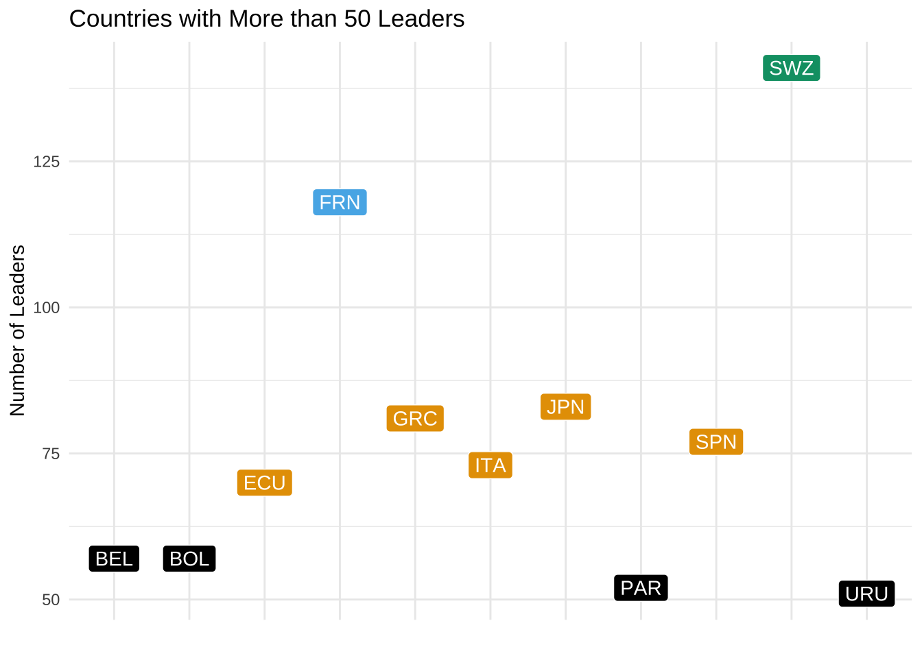
France, Greece, Japan, and Switzerland have had a large number of leaders during this period. All of the top 50 are in Europe or Latin America, save Japan. What does the overall data look like?
ggplot(data = Shorty) +
    aes(x = count) +
    geom_histogram(bins = 100, fill = '#9c179e') +
    labs(title = 'How Many Leaders since 1875?',
         x = 'Number of Leaders',
         y = 'Number of Countries',
         caption = 'data from Archigos') +
    theme_economist_white()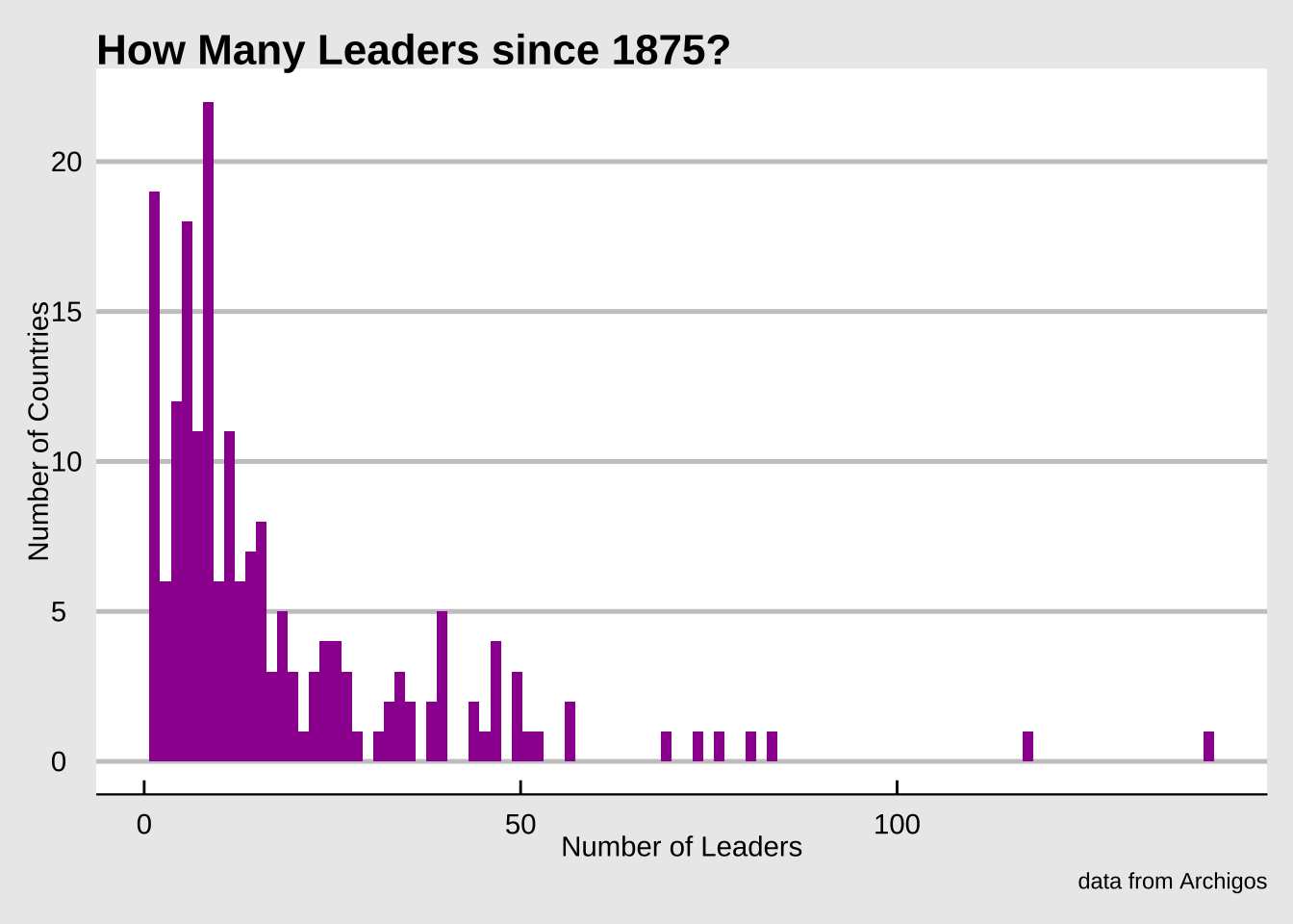
On Duration
Archigos %>% mutate(Duration = difftime(enddate, startdate, units="weeks")/52) %>% ggplot(aes(Duration)) + geom_histogram(bins=50, fill = '#9c179e') + theme_economist_white() + labs(y="Frequency", x="Tenure of Leader in Weeks [divided by 52]")## Don't know how to automatically pick scale for object of type difftime. Defaulting to continuous.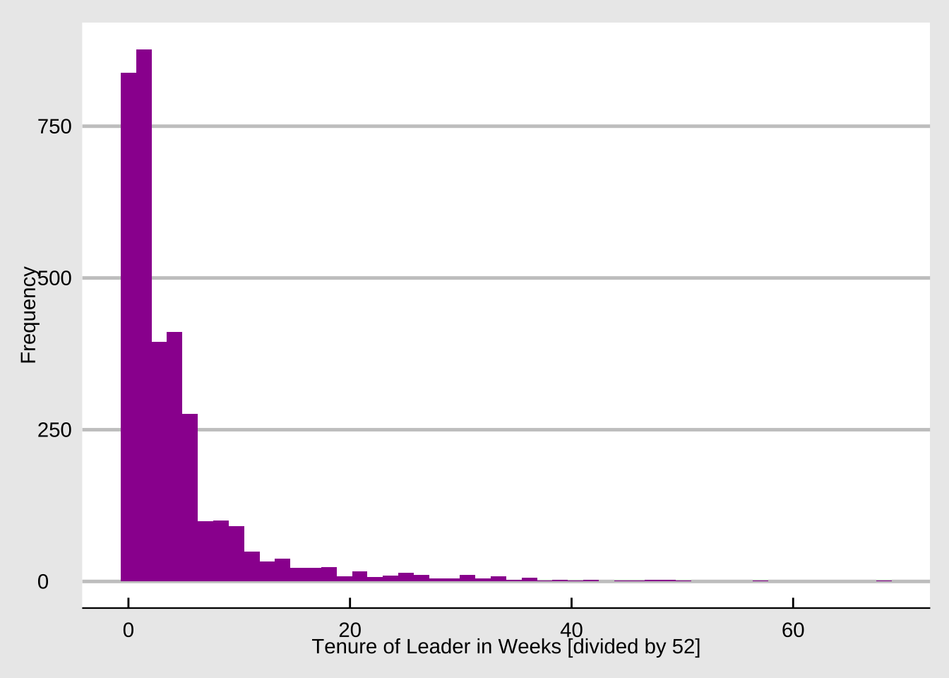
Who leads longest?
Archigos %>% mutate(Duration = difftime(enddate, startdate, units="weeks")) %>% select(leader,Duration) %>% arrange(desc(Duration)) %>% mutate(DurationInYears = Duration / 52)## # A tibble: 3,409 x 3
## leader Duration DurationInYears
## <chr> <drtn> <drtn>
## 1 Francis Joseph I 3546.429 weeks 68.20056 weeks
## 2 Nikola I Petrovic-Njegos 2944.286 weeks 56.62089 weeks
## 3 George I 2607.144 weeks 50.13738 weeks
## 4 Pedro II 2573.144 weeks 49.48353 weeks
## 5 Castro 2564.286 weeks 49.31319 weeks
## 6 Carol I 2524.572 weeks 48.54946 weeks
## 7 Hassanal Bolkiah 2517.149 weeks 48.40671 weeks
## 8 Nasir Ad-Din 2485.286 weeks 47.79397 weeks
## 9 Tz'u Hsi 2464.429 weeks 47.39287 weeks
## 10 Hussein Ibn Talal El-Hashim 2425.863 weeks 46.65121 weeks
## # … with 3,399 more rowsWhat happens to leaders?
The data includes the post tenure fate of all leaders. For now, I will take the data and build a bar graph of their fates as they are recorded.
Archigos %>% ggplot(., aes(posttenurefate)) + geom_bar(fill="purple") + coord_flip() + labs(y="Frequency", x="") + theme(axis.text.y = element_text(color = "purple", size = 8))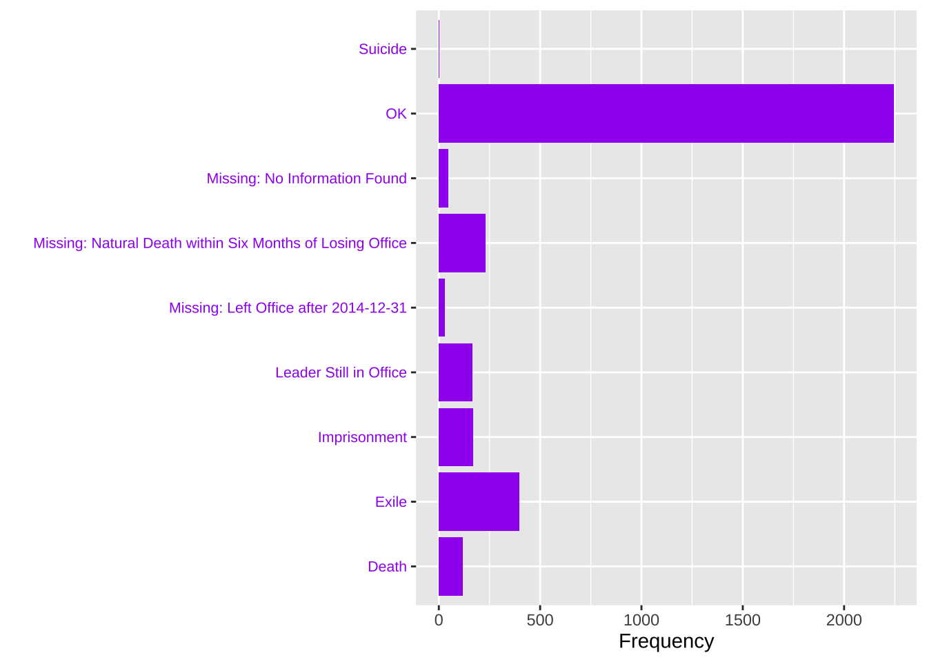
Discrete Annual Data
Now I want to analyse this as discrete data in annual form. I will use the lovely lubridate to extract the components of the date and then create a pivot table of sorts. It is important to note that there are a few problems here. There are some -999 values in the birth year.
Archigos <- Archigos %>% mutate(YearBorn = na_if(yrborn, -999))
Archigos <- Archigos %>% mutate(ExitAge = endYear - YearBorn)
How Old are Leaders When They Exit?
The smooth of these values is messy, but I will plot a simple static graph.
Archigos %>% filter(ExitAge > 12) %>% group_by(ExitAge) %>% summarise(countS=n()) %>% ggplot(., aes(x=ExitAge, y=countS))+ geom_point() + geom_smooth(method = "loess", span=0.25) + labs(title="Age at End of Tenure", x="Age in Years", y="Count") ## `geom_smooth()` using formula 'y ~ x'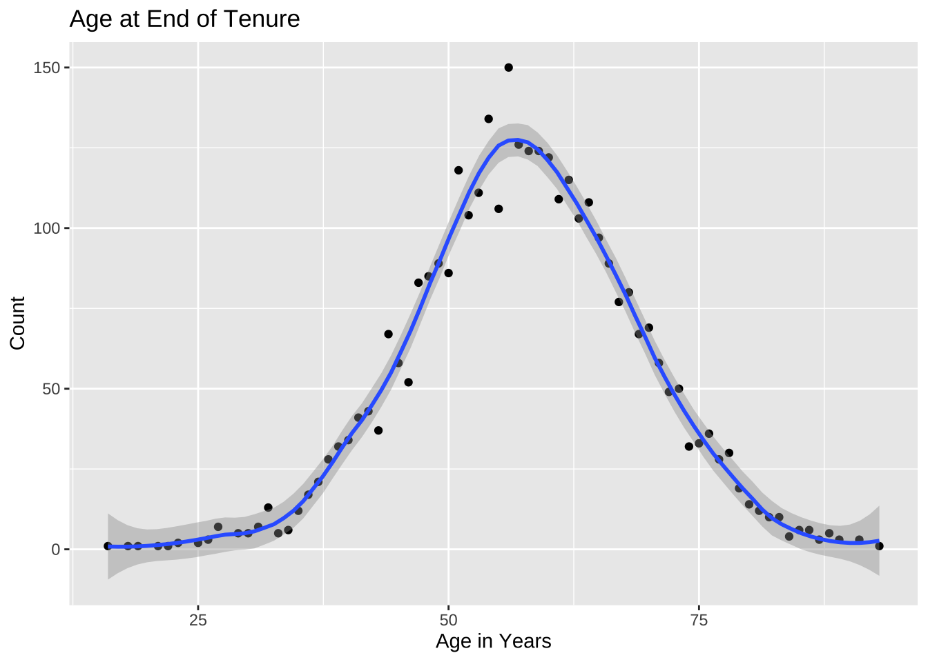
Or as a barplot.
Archigos %>% filter(ExitAge > 12) %>% ggplot(., aes(x=ExitAge, fill=cut_number(ExitAge, n=5))) + geom_bar() + scale_fill_viridis_d(guide=FALSE) + labs(title="Age at End of Tenure", x="Age in Years", y="Count") 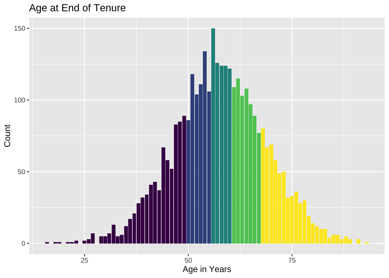
Yearly Turnovers
Now I can visualise turnovers on a yearly basis. NB: THis needs reworking.
YearlyD <- Archigos %>% group_by(endYear) %>% summarise(Endeds = n()) %>% filter(endYear < 2015)
YearlyD$label <- emoji("pencil2")
p <- YearlyD %>% ggplot(., aes(x=endYear, y=Endeds, label=label, colour="steelblue")) + geom_text(family="EmojiOne", size=10, position=position_nudge(x = 5, y = 5), color="steelblue") + geom_line(colour="steelblue") + theme_minimal() + labs(x="Year", y="Number of Leader-Tenures Ending")
panim <- p +  transition_reveal(endYear)
animate(panim, nframes=200)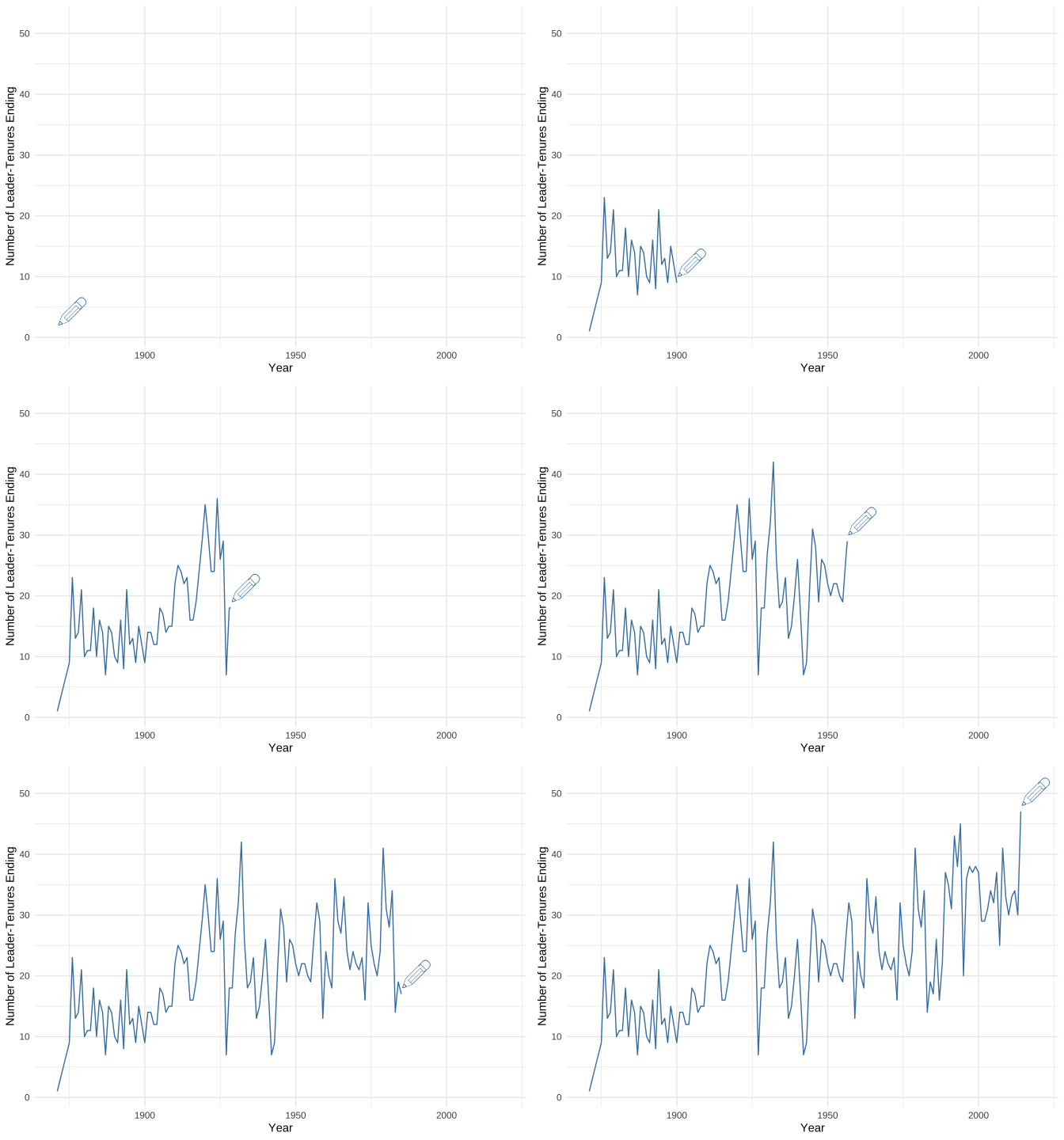
gganimate is a very neat tool. Now on to looking at what is happening at the country year and year level. In some ways, the previous is deceiving because the number of countries is widely varying over time. I build the country year and leader year data in the beginning. I will just recreate the Archigos version with the new variables that we have created in the interim.
Archigos <- Archigos %>% mutate(startYear = year(startdate), endYear = year(enddate))
DI <- dim(Archigos)[[1]]
tseq <-function(x) {
  tempd <- Archigos[x,]
  data.frame(obsid = tempd$obsid, leaderL = as.character(tempd$leader), leadidL = as.character(tempd$leadid), year=seq(tempd$startYear, tempd$endYear, by=1), LSY=tempd$startYear, LEY = tempd$endYear)
}
LTS <- lapply(seq(1,DI), function(x) { tseq(x) } )
LTS.Data <- data.frame(do.call(rbind, LTS))
LTS.Data$obsid <- as.character(LTS.Data$obsid)
Archigos$obsid <- as.character(Archigos$obsid)
Full.LTS <- LTS.Data %>% left_join(Archigos, by=c("obsid" = "obsid"))
# One curiosity; does any leader lead two distinct countries?  Having the ccodes allows me to calculate the standard deviation by leader.
So that gives me the basic country year dataset that defines the various existence years from countries. Neat. Now I need to create the leader year version of Archigos and merge it into my country year template for existence.
Full.LTS$Event <- (Full.LTS$year==Full.LTS$endYear)
Keepers <- Full.LTS %>% filter(year>1874 & year < 2015)
Shorty2 <- Keepers %>% group_by(year) %>% summarise(FailRate = mean(Event))
Shorty2$label <- emoji("pencil2")
p <- Shorty2 %>% ggplot(., aes(x=year, y=FailRate, label=label, colour='steelblue')) + geom_text(family="EmojiOne", size=10, position=position_nudge(x = 5, y = 0.03), color='steelblue') + geom_line(color='steelblue') + theme_minimal() + labs(x="Year", y="Proportion of Leaders Ending") + ylim(c(0,0.5))
panim <- p +  transition_reveal(year)
animate(panim, nframes=200)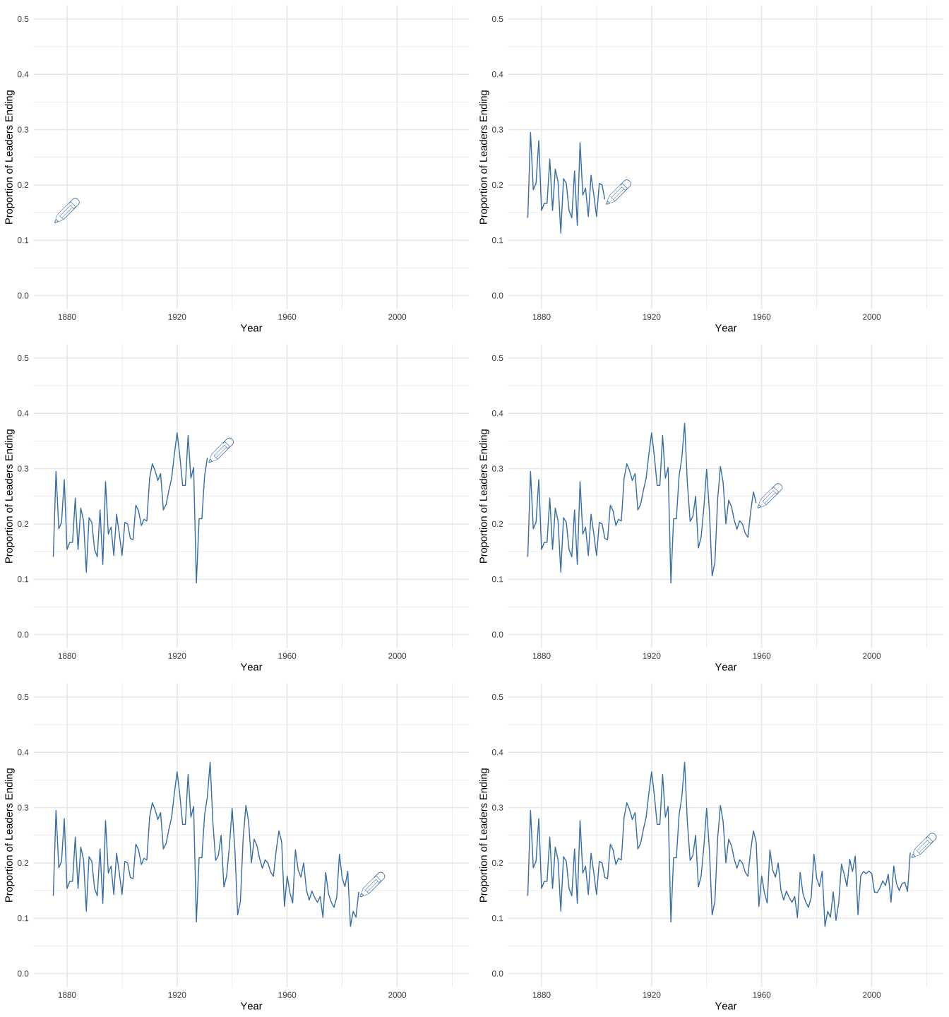
Averaging Turnover?
What if we decided to group the countries in the aforementioned data of Keepers and, instead, think about the cross-section nature of turnover?
library(ggrepel)
PlotSet <- Keepers %>% filter(year>1874 & year < 2015) %>% group_by(idacr) %>% summarise(Turnover.Pct = mean(Event)) %>% arrange(desc(Turnover.Pct)) %>% mutate(id=row_number(), facetID = cut_number(Turnover.Pct, n=4))
NameAbb <- iisystem %>% select(idacr, CountryName)
PlotSet <- PlotSet %>% left_join(NameAbb, by=c("idacr"="idacr"))
knitr::kable(PlotSet)| idacr | Turnover.Pct | id | facetID | CountryName |
|---|---|---|---|---|
| SWZ | 0.9929078 | 1 | (0.212,0.993] | Switzerland |
| BOS | 0.4791667 | 2 | (0.212,0.993] | Bosnia-Herzegovina |
| FRN | 0.4588235 | 3 | (0.212,0.993] | France |
| LAT | 0.4102564 | 4 | (0.212,0.993] | Latvia |
| LAT | 0.4102564 | 4 | (0.212,0.993] | Latvia |
| ZAN | 0.4000000 | 5 | (0.212,0.993] | Zanzibar |
| EST | 0.3947368 | 6 | (0.212,0.993] | Estonia |
| EST | 0.3947368 | 6 | (0.212,0.993] | Estonia |
| JPN | 0.3693694 | 7 | (0.212,0.993] | Japan |
| GRC | 0.3657407 | 8 | (0.212,0.993] | Greece |
| SPN | 0.3518519 | 9 | (0.212,0.993] | Spain |
| ITA | 0.3396226 | 10 | (0.212,0.993] | Italy/Sardinia |
| VIE | 0.3333333 | 11 | (0.212,0.993] | NA |
| ECU | 0.3301435 | 12 | (0.212,0.993] | Ecuador |
| RVN | 0.3225806 | 13 | (0.212,0.993] | Vietnam, Republic of |
| CZR | 0.3125000 | 14 | (0.212,0.993] | Czech Republic |
| BEL | 0.2931937 | 15 | (0.212,0.993] | Belgium |
| PAN | 0.2911392 | 16 | (0.212,0.993] | Panama |
| SOL | 0.2884615 | 17 | (0.212,0.993] | Solomon Islands |
| BOL | 0.2871795 | 18 | (0.212,0.993] | Bolivia |
| SLV | 0.2857143 | 19 | (0.212,0.993] | Slovenia |
| MAC | 0.2812500 | 20 | (0.212,0.993] | Macedonia (Former Yugoslav Republic of) |
| NOR | 0.2810458 | 21 | (0.212,0.993] | Norway |
| HAI | 0.2771084 | 22 | (0.212,0.993] | Haiti |
| HAI | 0.2771084 | 22 | (0.212,0.993] | Haiti |
| PAK | 0.2688172 | 23 | (0.212,0.993] | Pakistan |
| PAR | 0.2670157 | 24 | (0.212,0.993] | Paraguay |
| DOM | 0.2666667 | 25 | (0.212,0.993] | Dominican Republic |
| URU | 0.2592593 | 26 | (0.212,0.993] | Uruguay |
| ARG | 0.2553191 | 27 | (0.212,0.993] | Argentina |
| CHL | 0.2553191 | 28 | (0.212,0.993] | Chile |
| PER | 0.2473118 | 29 | (0.212,0.993] | Peru |
| COM | 0.2452830 | 30 | (0.212,0.993] | Comoros |
| GNB | 0.2452830 | 31 | (0.212,0.993] | Guinea-Bissau |
| ICE | 0.2446809 | 32 | (0.212,0.993] | Iceland |
| SAL | 0.2432432 | 33 | (0.212,0.993] | El Salvador |
| BNG | 0.2413793 | 34 | (0.212,0.993] | Bangladesh |
| COL | 0.2391304 | 35 | (0.212,0.993] | Colombia |
| ETM | 0.2352941 | 36 | (0.212,0.993] | East Timor |
| SWD | 0.2349727 | 37 | (0.212,0.993] | Sweden |
| GRG | 0.2258065 | 38 | (0.212,0.993] | Georgia |
| GMY | 0.2247191 | 39 | (0.212,0.993] | Germany (Prussia) |
| AUL | 0.2244898 | 40 | (0.212,0.993] | Australia |
| COS | 0.2191011 | 41 | (0.212,0.993] | Costa Rica |
| HON | 0.2178771 | 42 | (0.212,0.993] | Honduras |
| AUS | 0.2155172 | 43 | (0.212,0.993] | Austria |
| SLO | 0.2142857 | 44 | (0.212,0.993] | Slovakia |
| THI | 0.2134831 | 45 | (0.212,0.993] | Thailand |
| VEN | 0.2134831 | 46 | (0.212,0.993] | Venezuela |
| ALB | 0.2131148 | 47 | (0.212,0.993] | Albania |
| ISR | 0.2117647 | 48 | (0.146,0.212] | Israel |
| DEN | 0.2114286 | 49 | (0.146,0.212] | Denmark |
| BRA | 0.2102273 | 50 | (0.146,0.212] | Brazil |
| GUA | 0.2102273 | 51 | (0.146,0.212] | Guatemala |
| YPR | 0.2068966 | 52 | (0.146,0.212] | Yemen, People’s Republic of |
| OFS | 0.2045455 | 53 | (0.146,0.212] | Orange Free State |
| TRA | 0.2045455 | 54 | (0.146,0.212] | Transvaal |
| BEN | 0.2028986 | 55 | (0.146,0.212] | Benin |
| TUR | 0.2011494 | 56 | (0.146,0.212] | Turkey (Ottoman Empire) |
| AZE | 0.2000000 | 57 | (0.146,0.212] | Azerbaijan |
| IND | 0.2000000 | 58 | (0.146,0.212] | India |
| LAO | 0.2000000 | 59 | (0.146,0.212] | Laos |
| LIT | 0.2000000 | 60 | (0.146,0.212] | Lithuania |
| LIT | 0.2000000 | 60 | (0.146,0.212] | Lithuania |
| PNG | 0.2000000 | 61 | (0.146,0.212] | Papua New Guinea |
| NTH | 0.1964286 | 62 | (0.146,0.212] | Netherlands |
| MLD | 0.1935484 | 63 | (0.146,0.212] | Moldova |
| NIG | 0.1911765 | 64 | (0.146,0.212] | Nigeria |
| UKG | 0.1907514 | 65 | (0.146,0.212] | United Kingdom |
| IRE | 0.1880342 | 66 | (0.146,0.212] | Ireland |
| NIC | 0.1867470 | 67 | (0.146,0.212] | Nicaragua |
| NEP | 0.1860465 | 68 | (0.146,0.212] | Nepal |
| BUI | 0.1846154 | 69 | (0.146,0.212] | Burundi |
| FJI | 0.1818182 | 70 | (0.146,0.212] | Fiji |
| SYR | 0.1818182 | 71 | (0.146,0.212] | Syria |
| NEW | 0.1742424 | 72 | (0.146,0.212] | New Zealand |
| SIE | 0.1692308 | 73 | (0.146,0.212] | Sierra Leone |
| SUD | 0.1690141 | 74 | (0.146,0.212] | Sudan |
| YUG | 0.1683168 | 75 | (0.146,0.212] | Yugoslavia |
| MAA | 0.1666667 | 76 | (0.146,0.212] | Mauritania |
| SUR | 0.1666667 | 77 | (0.146,0.212] | Surinam |
| UKR | 0.1666667 | 78 | (0.146,0.212] | Ukraine |
| HUN | 0.1652174 | 79 | (0.146,0.212] | Hungary |
| POL | 0.1636364 | 80 | (0.146,0.212] | Poland |
| LEB | 0.1627907 | 81 | (0.146,0.212] | Lebanon |
| AFG | 0.1626506 | 82 | (0.146,0.212] | Afghanistan |
| AFG | 0.1626506 | 82 | (0.146,0.212] | Afghanistan |
| ROK | 0.1625000 | 83 | (0.146,0.212] | Korea, Republic of |
| SRI | 0.1625000 | 84 | (0.146,0.212] | Sri Lanka (Ceylon) |
| SER | 0.1600000 | 85 | (0.146,0.212] | Serbia |
| SER | 0.1600000 | 85 | (0.146,0.212] | Serbia |
| JAM | 0.1587302 | 86 | (0.146,0.212] | Jamaica |
| USA | 0.1566265 | 87 | (0.146,0.212] | NA |
| BFO | 0.1538462 | 88 | (0.146,0.212] | Burkina Faso (Upper Volta) |
| IRQ | 0.1530612 | 89 | (0.146,0.212] | Iraq |
| MEX | 0.1524390 | 90 | (0.146,0.212] | Mexico |
| BUL | 0.1523179 | 91 | (0.146,0.212] | Bulgaria |
| CAN | 0.1515152 | 92 | (0.146,0.212] | Canada |
| CZE | 0.1494253 | 93 | (0.146,0.212] | Czechoslovakia |
| GHA | 0.1486486 | 94 | (0.146,0.212] | Ghana |
| MYA | 0.1428571 | 95 | (0.0844,0.146] | Myanmar (Burma) |
| MYA | 0.1428571 | 95 | (0.0844,0.146] | Myanmar (Burma) |
| VNM | 0.1428571 | 96 | (0.0844,0.146] | Vietnam (Annam/Cochin China/Tonkin) |
| LBR | 0.1419753 | 97 | (0.0844,0.146] | Liberia |
| RUM | 0.1419753 | 98 | (0.0844,0.146] | Rumania |
| CYP | 0.1406250 | 99 | (0.0844,0.146] | Cyprus |
| SAF | 0.1393443 | 100 | (0.0844,0.146] | South Africa |
| CRO | 0.1379310 | 101 | (0.0844,0.146] | Croatia |
| CHN | 0.1366460 | 102 | (0.0844,0.146] | China |
| BHU | 0.1359223 | 103 | (0.0844,0.146] | Bhutan |
| CUB | 0.1338583 | 104 | (0.0844,0.146] | Cuba |
| ALG | 0.1311475 | 105 | (0.0844,0.146] | Algeria |
| ALG | 0.1311475 | 105 | (0.0844,0.146] | Algeria |
| MAG | 0.1279070 | 106 | (0.0844,0.146] | Madagascar (Malagasy) |
| MAG | 0.1279070 | 106 | (0.0844,0.146] | Madagascar |
| CEN | 0.1269841 | 107 | (0.0844,0.146] | Central African Republic |
| NIR | 0.1269841 | 108 | (0.0844,0.146] | Niger |
| PHI | 0.1265823 | 109 | (0.0844,0.146] | Philippines |
| BAR | 0.1250000 | 110 | (0.0844,0.146] | Barbados |
| KOS | 0.1250000 | 111 | (0.0844,0.146] | Kosovo |
| LES | 0.1250000 | 112 | (0.0844,0.146] | Lesotho |
| POR | 0.1250000 | 113 | (0.0844,0.146] | Portugal |
| LUX | 0.1233766 | 114 | (0.0844,0.146] | Luxembourg |
| MON | 0.1214953 | 115 | (0.0844,0.146] | Mongolia |
| FIN | 0.1171171 | 116 | (0.0844,0.146] | Finland |
| MLT | 0.1166667 | 117 | (0.0844,0.146] | Malta |
| UGA | 0.1166667 | 118 | (0.0844,0.146] | Uganda |
| INS | 0.1139241 | 119 | (0.0844,0.146] | Indonesia |
| MAS | 0.1132075 | 120 | (0.0844,0.146] | Mauritius |
| CON | 0.1129032 | 121 | (0.0844,0.146] | Congo |
| MLI | 0.1129032 | 122 | (0.0844,0.146] | Mali |
| BHM | 0.1111111 | 123 | (0.0844,0.146] | Bahamas |
| BLR | 0.1111111 | 124 | (0.0844,0.146] | Belarus (Byelorussia) |
| TAJ | 0.1111111 | 125 | (0.0844,0.146] | Tajikistan |
| GUY | 0.1090909 | 126 | (0.0844,0.146] | Guyana |
| MAL | 0.1076923 | 127 | (0.0844,0.146] | Malaysia |
| KYR | 0.1071429 | 128 | (0.0844,0.146] | Kyrgyz Republic |
| GDR | 0.1020408 | 129 | (0.0844,0.146] | German Democratic Republic |
| TRI | 0.1016949 | 130 | (0.0844,0.146] | Trinidad and Tobago |
| LIB | 0.0985915 | 131 | (0.0844,0.146] | Libya |
| LIB | 0.0985915 | 131 | (0.0844,0.146] | Libya |
| TOG | 0.0983607 | 132 | (0.0844,0.146] | Togo |
| GFR | 0.0958904 | 133 | (0.0844,0.146] | German Federal Republic |
| GUI | 0.0952381 | 134 | (0.0844,0.146] | Guinea |
| DRV | 0.0909091 | 135 | (0.0844,0.146] | Vietnam, Democratic Republic of |
| ZAM | 0.0892857 | 136 | (0.0844,0.146] | Zambia |
| CAM | 0.0882353 | 137 | (0.0844,0.146] | Cambodia (Kampuchea) |
| EGY | 0.0882353 | 138 | (0.0844,0.146] | Egypt |
| EGY | 0.0882353 | 138 | (0.0844,0.146] | Egypt |
| KUW | 0.0857143 | 139 | (0.0844,0.146] | Kuwait |
| IRN | 0.0849673 | 140 | (0.0844,0.146] | Iran (Persia) |
| BLZ | 0.0847458 | 141 | (0.0844,0.146] | Belize |
| DRC | 0.0833333 | 142 | [0,0.0844] | Congo, Democratic Republic of (Zaire) |
| GAB | 0.0833333 | 143 | [0,0.0844] | Gabon |
| TAW | 0.0833333 | 144 | [0,0.0844] | Taiwan |
| TUN | 0.0813953 | 145 | [0,0.0844] | Tunisia |
| TUN | 0.0813953 | 145 | [0,0.0844] | Tunisia |
| SOM | 0.0810811 | 146 | [0,0.0844] | Somalia |
| RUS | 0.0794702 | 147 | [0,0.0844] | Russia (Soviet Union) |
| ETH | 0.0789474 | 148 | [0,0.0844] | Ethiopia |
| ARM | 0.0769231 | 149 | [0,0.0844] | Armenia |
| YEM | 0.0750000 | 150 | [0,0.0844] | Yemen (Arab Republic of Yemen) |
| MAD | 0.0746269 | 151 | [0,0.0844] | Maldives |
| TBT | 0.0731707 | 152 | [0,0.0844] | Tibet |
| MAW | 0.0727273 | 153 | [0,0.0844] | Malawi |
| CAP | 0.0697674 | 154 | [0,0.0844] | Cape Verde |
| CDI | 0.0677966 | 155 | [0,0.0844] | Ivory Coast |
| CHA | 0.0677966 | 156 | [0,0.0844] | Chad |
| QAT | 0.0638298 | 157 | [0,0.0844] | Qatar |
| SWA | 0.0600000 | 158 | [0,0.0844] | Swaziland |
| BOT | 0.0576923 | 159 | [0,0.0844] | Botswana |
| KEN | 0.0545455 | 160 | [0,0.0844] | Kenya |
| KOR | 0.0540541 | 161 | [0,0.0844] | Korea |
| SAU | 0.0537634 | 162 | [0,0.0844] | Saudi Arabia |
| RWA | 0.0526316 | 163 | [0,0.0844] | Rwanda |
| SEN | 0.0526316 | 164 | [0,0.0844] | Senegal |
| TAZ | 0.0526316 | 165 | [0,0.0844] | Tanzania/Tanganyika |
| MZM | 0.0476190 | 166 | [0,0.0844] | Mozambique |
| AUH | 0.0444444 | 167 | [0,0.0844] | Austria-Hungary |
| MOR | 0.0416667 | 168 | [0,0.0844] | Morocco |
| MOR | 0.0416667 | 168 | [0,0.0844] | Morocco |
| JOR | 0.0408163 | 169 | [0,0.0844] | Jordan |
| ZIM | 0.0392157 | 170 | [0,0.0844] | Zimbabwe (Rhodesia) |
| NAM | 0.0384615 | 171 | [0,0.0844] | Namibia |
| TKM | 0.0384615 | 172 | [0,0.0844] | Turkmenistan |
| EQG | 0.0370370 | 173 | [0,0.0844] | Equatorial Guinea |
| SIN | 0.0344828 | 174 | [0,0.0844] | Singapore |
| PRK | 0.0289855 | 175 | [0,0.0844] | Korea, People’s Republic of |
| OMA | 0.0277778 | 176 | [0,0.0844] | Oman |
| DJI | 0.0256410 | 177 | [0,0.0844] | Djibouti |
| ANG | 0.0243902 | 178 | [0,0.0844] | Angola |
| MNG | 0.0232558 | 179 | [0,0.0844] | Montenegro |
| MNG | 0.0232558 | 179 | [0,0.0844] | Montenegro |
| BAH | 0.0222222 | 180 | [0,0.0844] | Bahrain |
| UAE | 0.0222222 | 181 | [0,0.0844] | United Arab Emirates |
| GAM | 0.0196078 | 182 | [0,0.0844] | Gambia |
| CAO | 0.0178571 | 183 | [0,0.0844] | Cameroon |
| BRU | 0.0000000 | 184 | [0,0.0844] | Brunei |
| ERI | 0.0000000 | 185 | [0,0.0844] | Eritrea |
| KZK | 0.0000000 | 186 | [0,0.0844] | Kazakhstan |
| SSD | 0.0000000 | 187 | [0,0.0844] | South Sudan |
| UZB | 0.0000000 | 188 | [0,0.0844] | Uzbekistan |
Now a picture.
PlotSet %>% ggplot(., aes(x=Turnover.Pct)) + geom_histogram(fill="purple", binwidth=0.05) + ggtitle("Turnover by Country")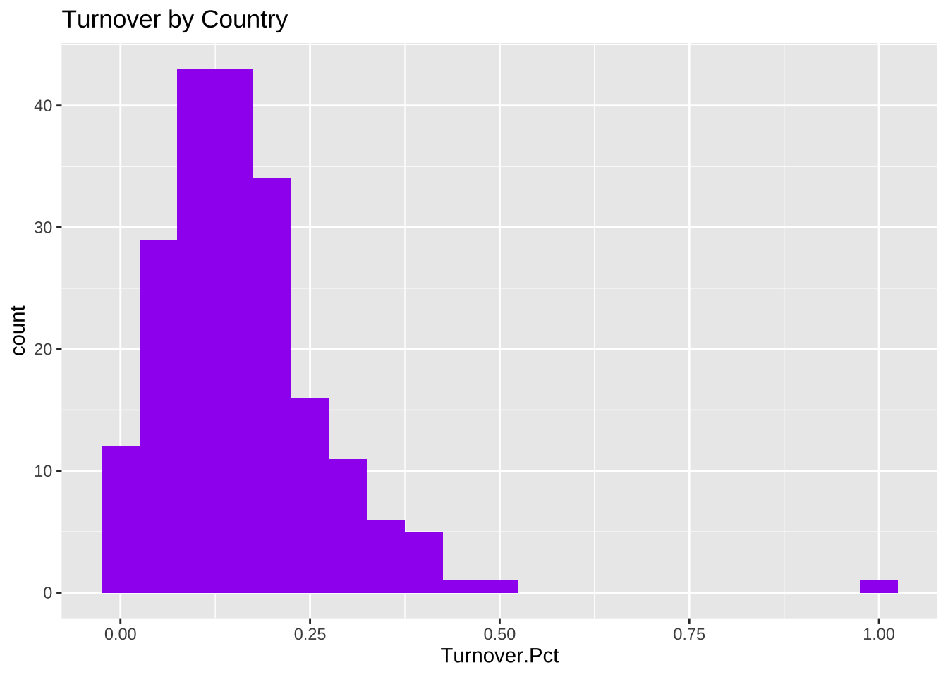
Switzerland turnover is 1.
The Fun Stuff: Durations
Richard Tucker did some work on binary time series cross section data for their paper 20! years ago [his with Neal Beck, Jonathan Katz]. David Armstrong’s btscs takes a binary time series and turns it into a set of discrete time durations. Grouped duration data is their name for it. There’s a rather neat stats feature to the fact that these grouped duration data are exactly the same as a discrete time Cox proportional hazards model. In a related paper, two of the most clever people that I know – David Carter and Curt Signorino – showed that a Taylor-series approximation to the cubic polynomial in that duration approximates just about anything reasonable because it can embed two inflection points for the baseline hazard. Of course, there are assumptions to the model but let’s explore. First, a static picture.
Even easier
It turns out that the leader-year data have duration data embedded in them. Two conditions create the data that we need. First, the actual duration is created by taking calendar year minus startYear. Second, the events are one if calendar year is equal to endYear. Plus, leader-spells are properly nested in countries so we can measure this easily.
Full.LTS$spell <- Full.LTS$year - Full.LTS$startYear
p <- Full.LTS %>% filter(!is.na(posttenurefate)) %>% mutate(howEndedF = factor(posttenurefate)) %>% ggplot(aes(x=spell)) + geom_density(aes(color=howEndedF)) + scale_color_viridis_d(guide=FALSE)+ theme_minimal() + labs(title="How Long Do Leaders Last Given Fates?", x="Leader Duration in Years")
p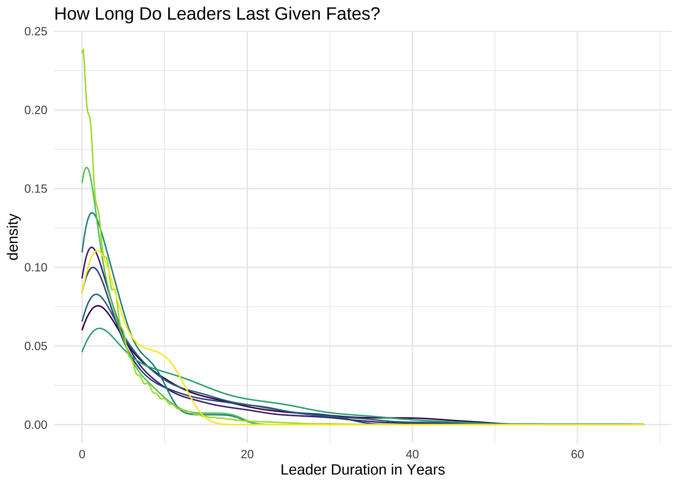
Animate it.
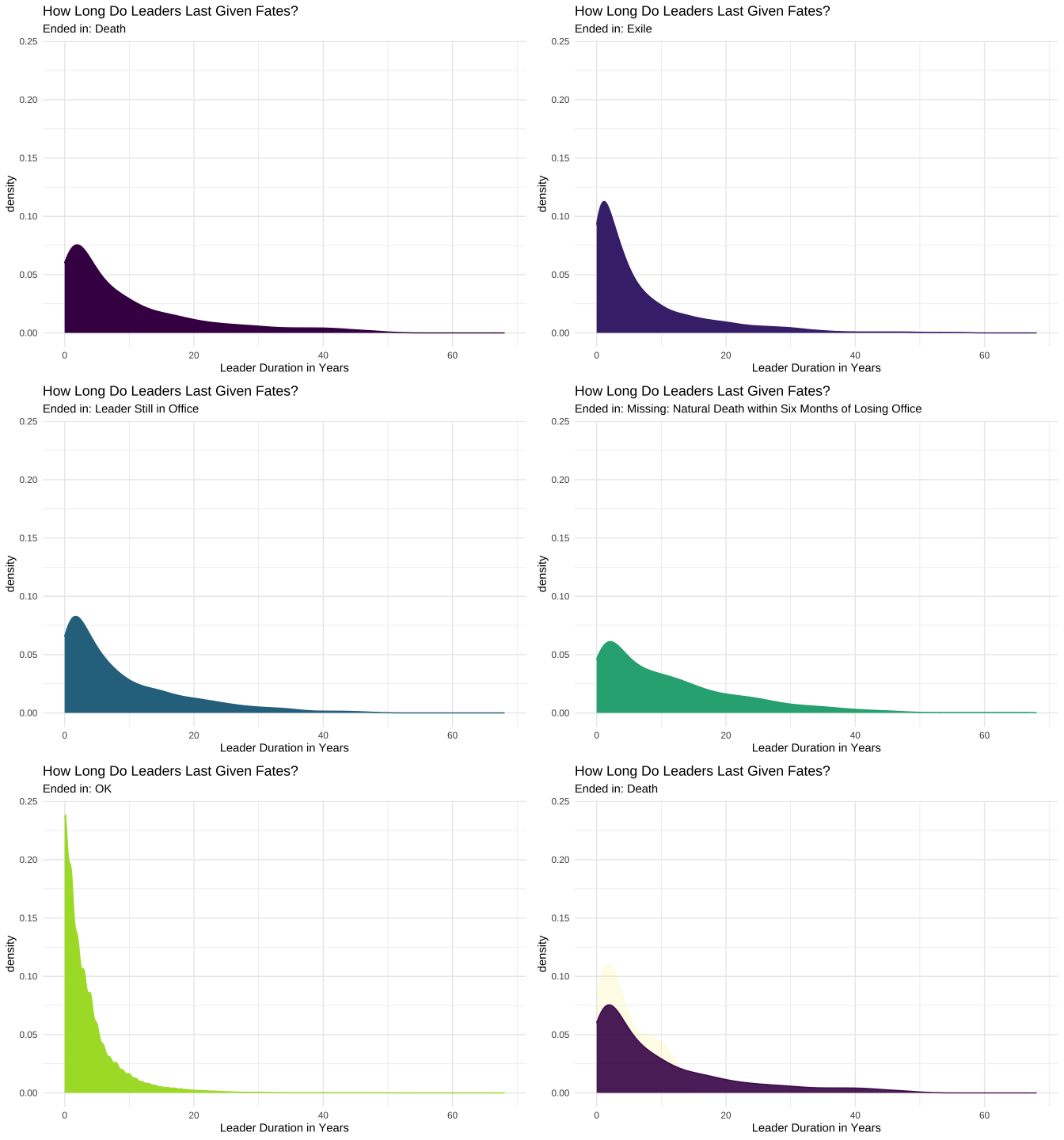
panim <- Full.LTS %>% filter(!is.na(posttenurefate)) %>% mutate(howEndedF = factor(posttenurefate)) %>% ggplot(aes(x=spell)) + geom_density(aes(color=howEndedF, fill=howEndedF)) + scale_color_viridis_d(guide=FALSE) + scale_fill_viridis_d(guide=FALSE) + theme_minimal() + labs(title="How Long Do Leaders Last Given Fates?", subtitle = "Ended in: {closest_state}", x="Leader Duration in Years") + transition_states(howEndedF, transition_length = 10, state_length = 40) + enter_fade() + exit_fade()
animate(panim, nframes=400)